Chapter 3 The Greedy Method 4 1 The

Chapter 3 The Greedy Method 4 -1

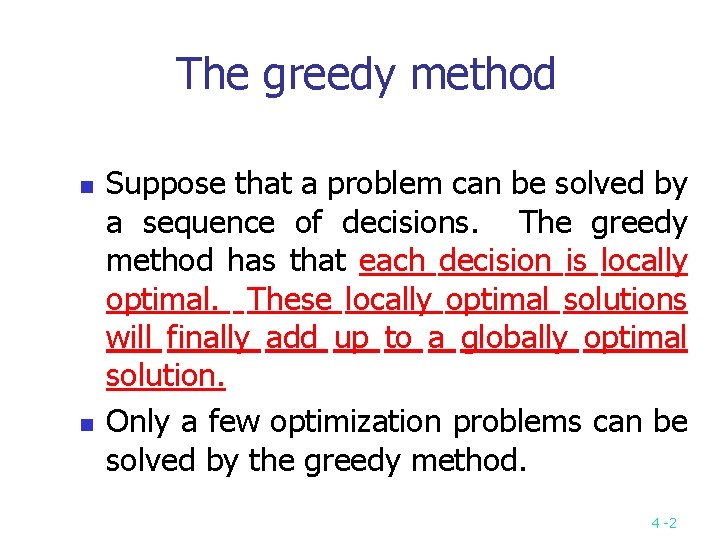
The greedy method n n Suppose that a problem can be solved by a sequence of decisions. The greedy method has that each decision is locally optimal. These locally optimal solutions will finally add up to a globally optimal solution. Only a few optimization problems can be solved by the greedy method. 4 -2

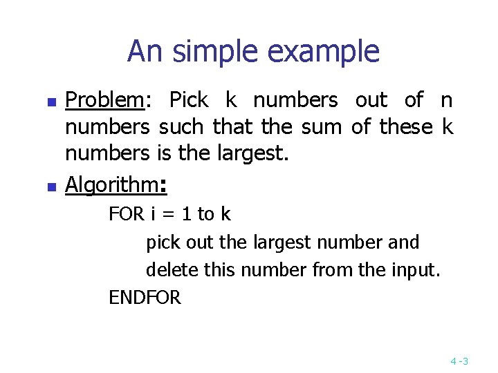
An simple example n n Problem: Pick k numbers out of n numbers such that the sum of these k numbers is the largest. Algorithm: FOR i = 1 to k pick out the largest number and delete this number from the input. ENDFOR 4 -3

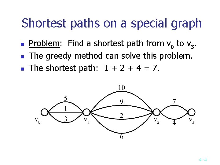
Shortest paths on a special graph n n n Problem: Find a shortest path from v 0 to v 3. The greedy method can solve this problem. The shortest path: 1 + 2 + 4 = 7. 4 -4

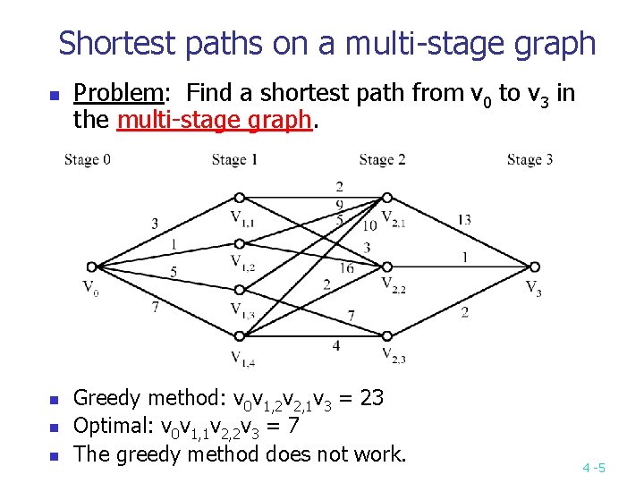
Shortest paths on a multi-stage graph n n Problem: Find a shortest path from v 0 to v 3 in the multi-stage graph. Greedy method: v 0 v 1, 2 v 2, 1 v 3 = 23 Optimal: v 0 v 1, 1 v 2, 2 v 3 = 7 The greedy method does not work. 4 -5

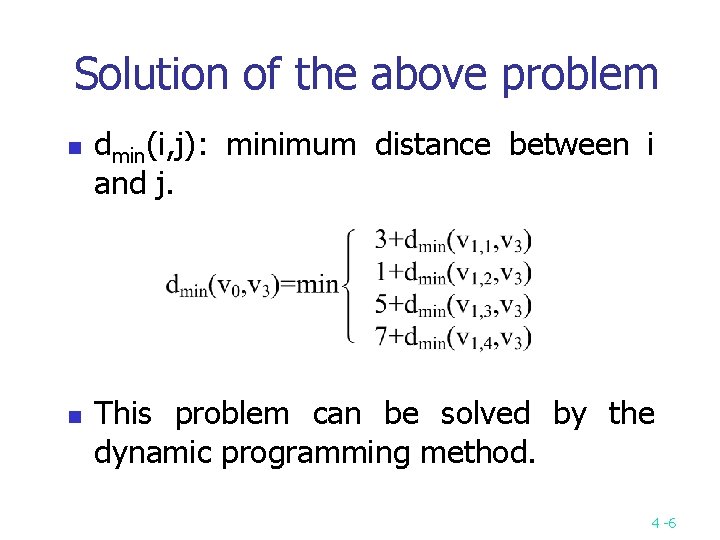
Solution of the above problem n n dmin(i, j): minimum distance between i and j. This problem can be solved by the dynamic programming method. 4 -6

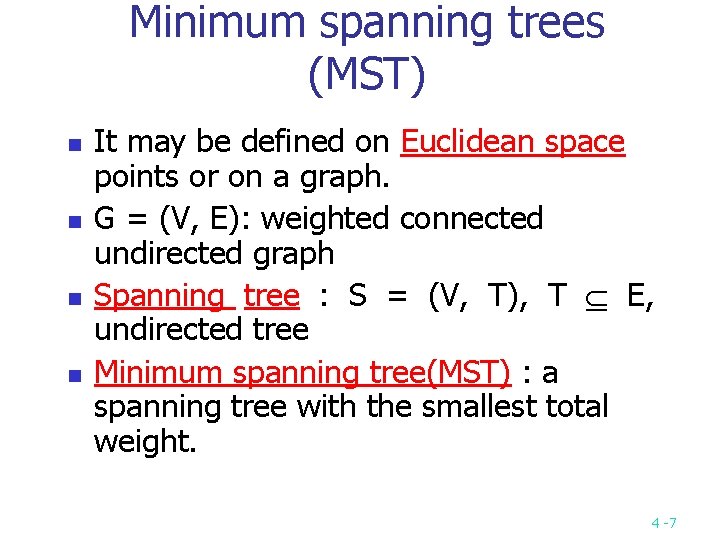
Minimum spanning trees (MST) n n It may be defined on Euclidean space points or on a graph. G = (V, E): weighted connected undirected graph Spanning tree : S = (V, T), T E, undirected tree Minimum spanning tree(MST) : a spanning tree with the smallest total weight. 4 -7

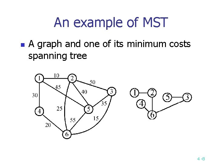
An example of MST n A graph and one of its minimum costs spanning tree 4 -8

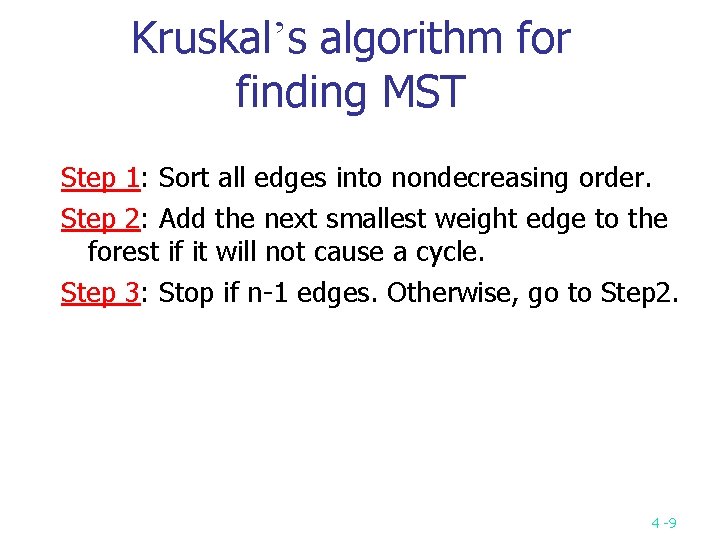
Kruskal’s algorithm for finding MST Step 1: Sort all edges into nondecreasing order. Step 2: Add the next smallest weight edge to the forest if it will not cause a cycle. Step 3: Stop if n-1 edges. Otherwise, go to Step 2. 4 -9

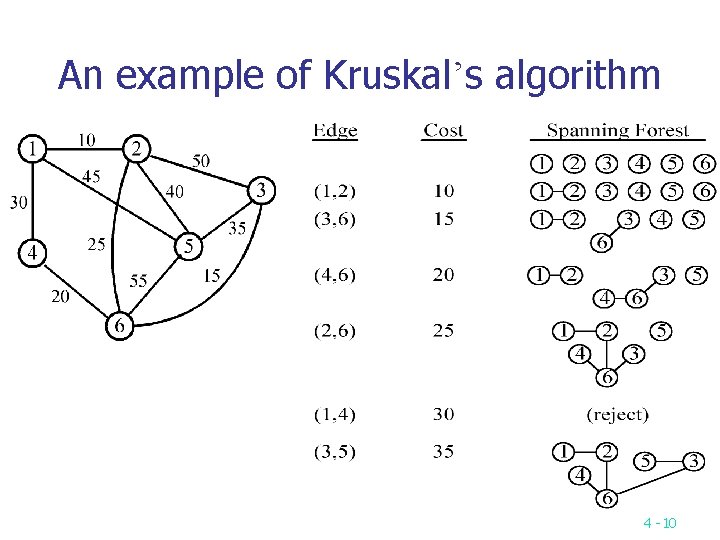
An example of Kruskal’s algorithm 4 -10

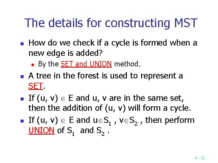
The details for constructing MST n How do we check if a cycle is formed when a new edge is added? n n By the SET and UNION method. A tree in the forest is used to represent a SET. If (u, v) E and u, v are in the same set, then the addition of (u, v) will form a cycle. If (u, v) E and u S 1 , v S 2 , then perform UNION of S 1 and S 2. 4 -11

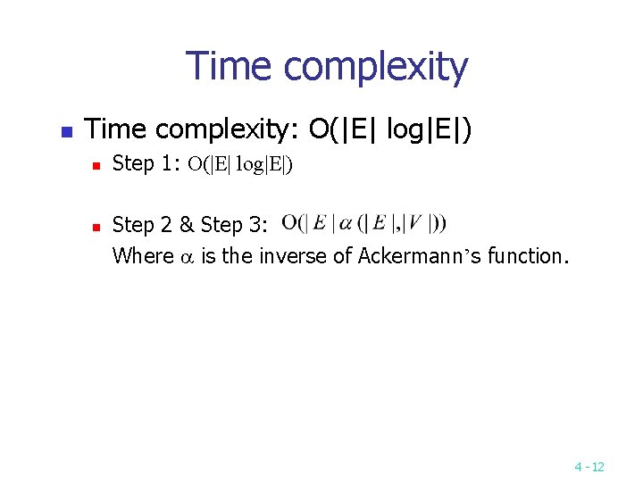
Time complexity n Time complexity: O(|E| log|E|) n n Step 1: O(|E| log|E|) Step 2 & Step 3: Where is the inverse of Ackermann’s function. 4 -12

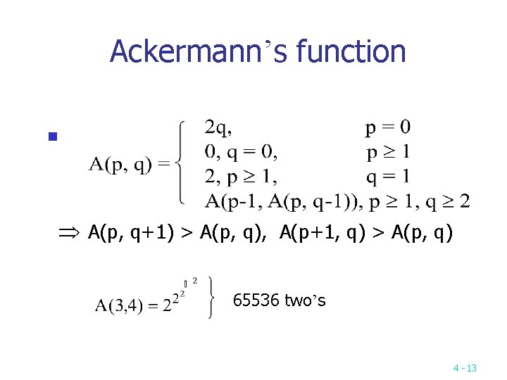
Ackermann’s function n A(p, q+1) > A(p, q), A(p+1, q) > A(p, q) 65536 two’s 4 -13

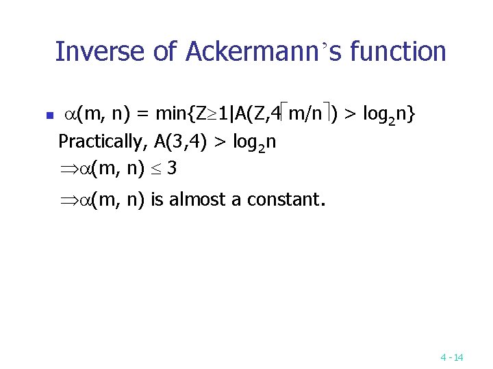
Inverse of Ackermann’s function n (m, n) = min{Z 1|A(Z, 4 m/n ) > log 2 n} Practically, A(3, 4) > log 2 n (m, n) 3 (m, n) is almost a constant. 4 -14

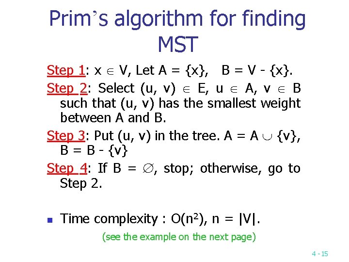
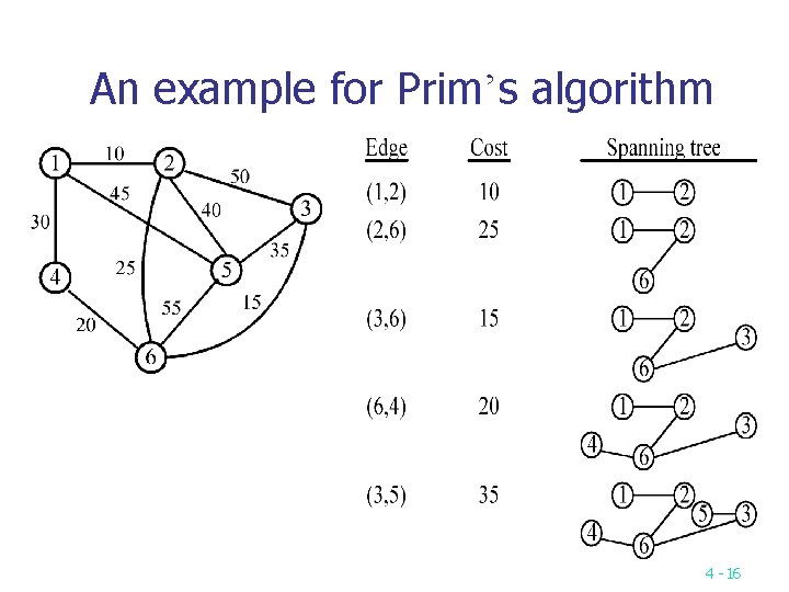
Prim’s algorithm for finding MST Step 1: x V, Let A = {x}, B = V - {x}. Step 2: Select (u, v) E, u A, v B such that (u, v) has the smallest weight between A and B. Step 3: Put (u, v) in the tree. A = A {v}, B = B - {v} Step 4: If B = , stop; otherwise, go to Step 2. n Time complexity : O(n 2), n = |V|. (see the example on the next page) 4 -15

An example for Prim’s algorithm 4 -16

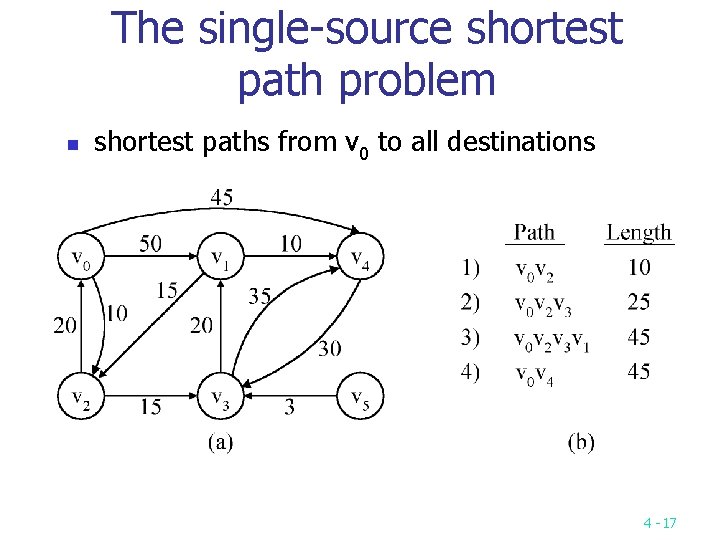
The single-source shortest path problem n shortest paths from v 0 to all destinations 4 -17

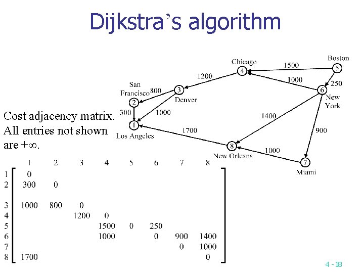
Dijkstra’s algorithm Cost adjacency matrix. All entries not shown are +. 4 -18

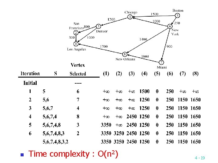
n Time complexity : O(n 2) 4 -19

The longest path problem n n Can we use Dijkstra’s algorithm to find the longest path from a starting vertex to an ending vertex in an acyclic directed graph? There are 3 possible ways to apply Dijkstra’s algorithm: n n Directly use “max” operations instead of “min” operations. Convert all positive weights to be negative. Then find the shortest path. Give a very large positive number M. If the weight of an edge is w, now M-w is used to replace w. Then find the shortest path. All these 3 possible ways would not work! 4 -20

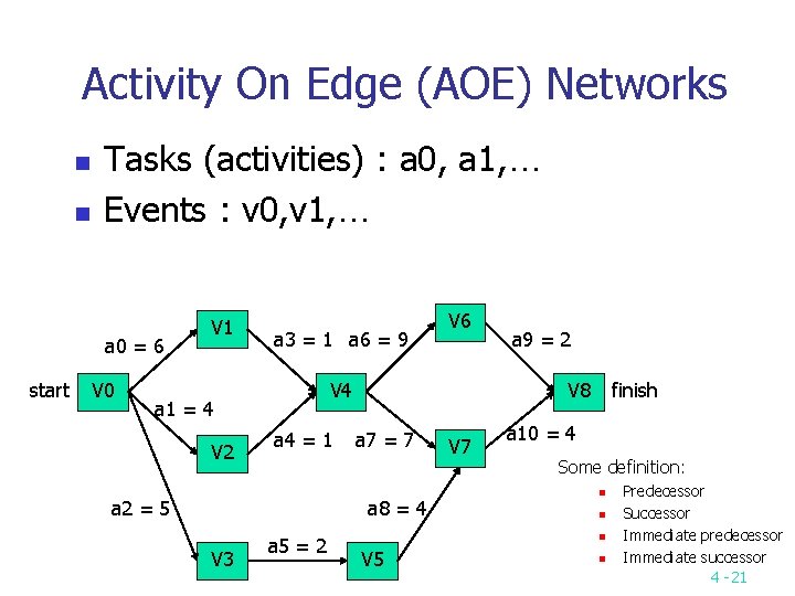
Activity On Edge (AOE) Networks n n Tasks (activities) : a 0, a 1, … Events : v 0, v 1, … a 0 = 6 start V 0 V 1 a 3 = 1 a 6 = 9 V 4 a 1 = 4 V 2 a 4 = 1 a 2 = 5 a 5 = 2 a 9 = 2 V 8 a 7 = 7 a 8 = 4 V 3 V 6 V 7 finish a 10 = 4 Some definition: n n n V 5 n Predecessor Successor Immediate predecessor Immediate successor 4 -21

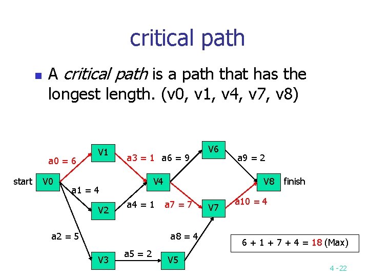
critical path n A critical path is a path that has the longest length. (v 0, v 1, v 4, v 7, v 8) a 0 = 6 start V 0 V 1 a 3 = 1 a 6 = 9 V 4 a 1 = 4 V 2 a 4 = 1 a 2 = 5 a 5 = 2 a 9 = 2 V 8 a 7 = 7 a 8 = 4 V 3 V 6 V 5 V 7 finish a 10 = 4 6 + 1 + 7 + 4 = 18 (Max) 4 -22

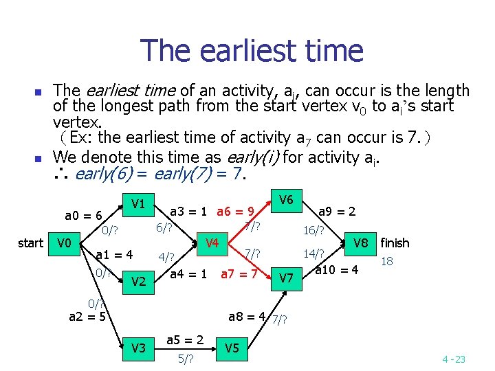
The earliest time n n The earliest time of an activity, ai, can occur is the length of the longest path from the start vertex v 0 to ai’s start vertex. （Ex: the earliest time of activity a 7 can occur is 7. ） We denote this time as early(i) for activity ai. ∴ early(6) = early(7) = 7. V 1 a 0 = 6 start V 0 7/? 6/? 0/? a 1 = 4 0/? a 3 = 1 a 6 = 9 V 2 V 6 V 4 a 4 = 1 0/? a 2 = 5 16/? 7/? 4/? a 7 = 7 a 9 = 2 14/? V 7 V 8 a 10 = 4 finish 18 a 8 = 4 7/? V 3 a 5 = 2 5/? V 5 4 -23

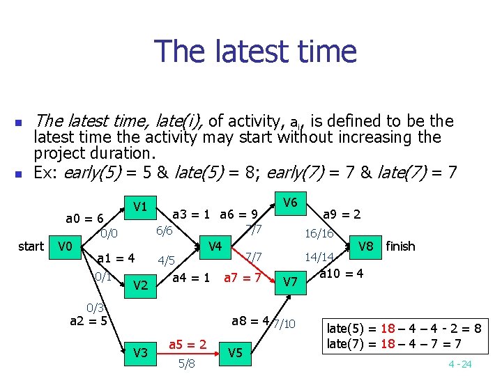
The latest time n n The latest time, late(i), of activity, ai, is defined to be the latest time the activity may start without increasing the project duration. Ex: early(5) = 5 & late(5) = 8; early(7) = 7 & late(7) = 7 a 0 = 6 start V 0 V 1 a 3 = 1 a 6 = 9 7/7 0/0 6/6 a 1 = 4 4/5 0/1 V 2 V 6 V 4 a 4 = 1 0/3 a 2 = 5 16/16 7/7 a 7 = 7 14/14 V 7 a 8 = 4 7/10 V 3 a 5 = 2 5/8 V 5 a 9 = 2 V 8 finish a 10 = 4 late(5) = 18 – 4 - 2 = 8 late(7) = 18 – 4 – 7 = 7 4 -24

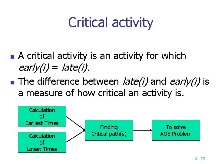
Critical activity n n A critical activity is an activity for which early(i) = late(i). The difference between late(i) and early(i) is a measure of how critical an activity is. Calculation of Earliest Times Calculation of Latest Times Finding Critical path(s) To solve AOE Problem 4 -25

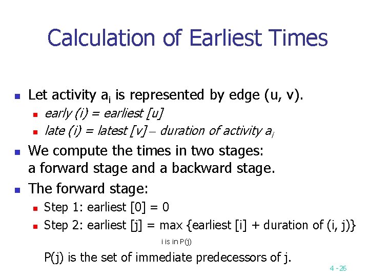
Calculation of Earliest Times n Let activity ai is represented by edge (u, v). n n early (i) = earliest [u] late (i) = latest [v] – duration of activity ai We compute the times in two stages: a forward stage and a backward stage. The forward stage: n n Step 1: earliest [0] = 0 Step 2: earliest [j] = max {earliest [i] + duration of (i, j)} i is in P(j) is the set of immediate predecessors of j. 4 -26

Calculation of Latest Times n The backward stage: n n Step 1: latest[n-1] = earliest[n-1] Step 2: latest [j] = min {latest [i] - duration of (j, i)} i is in S(j) is the set of vertices adjacent from vertex j. latest[8] latest[6] latest[7] latest[4] latest[1] latest[2] latest[5] latest[3] latest[0] = = = = = earliest[8] = 18 min{earliest[8] - 2} = 16 min{earliest[8] - 4} = 14 min{earliest[6] – 9; earliest[7] – 7} = 7 min{earliest[4] - 1} = 6 min{earliest[7] - 4} = 10 min{earliest[5] - 2} = 8 min{earliest[1] – 6; earliest[2] – 4; earliest[3] – 5} = 0 4 -27

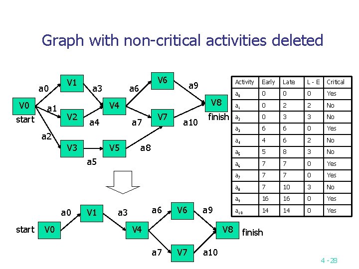
Graph with non-critical activities deleted a 0 V 0 a 1 start V 1 a 3 V 6 a 9 V 8 V 4 V 2 a 4 a 7 V 7 a 10 finish a 2 V 3 V 5 a 8 a 5 a 0 start V 0 V 1 a 6 a 3 V 6 a 9 V 4 V 8 a 7 V 7 a 10 Activity Early Late L-E Critical a 0 0 Yes a 1 0 2 2 No a 2 0 3 3 No a 3 6 6 0 Yes a 4 4 6 2 No a 5 5 8 3 No a 6 7 7 0 Yes a 7 7 7 0 Yes a 8 7 10 3 No a 9 16 16 0 Yes a 10 14 14 0 Yes finish 4 -28

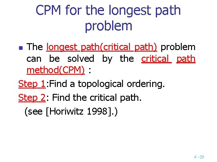
CPM for the longest path problem The longest path(critical path) problem can be solved by the critical path method(CPM) : Step 1: Find a topological ordering. Step 2: Find the critical path. (see [Horiwitz 1998]. ) n 4 -29

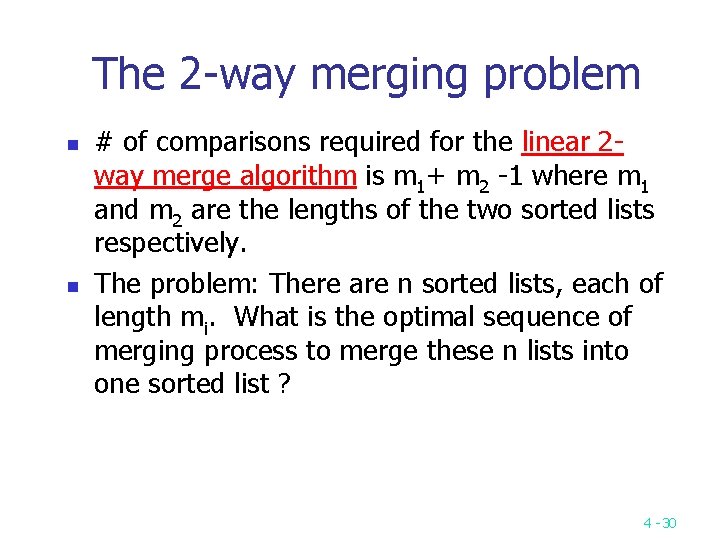
The 2 -way merging problem n n # of comparisons required for the linear 2 way merge algorithm is m 1+ m 2 -1 where m 1 and m 2 are the lengths of the two sorted lists respectively. The problem: There are n sorted lists, each of length mi. What is the optimal sequence of merging process to merge these n lists into one sorted list ? 4 -30

Extended binary trees n Extended Binary Tree Representing a 2 -way Merge 4 -31

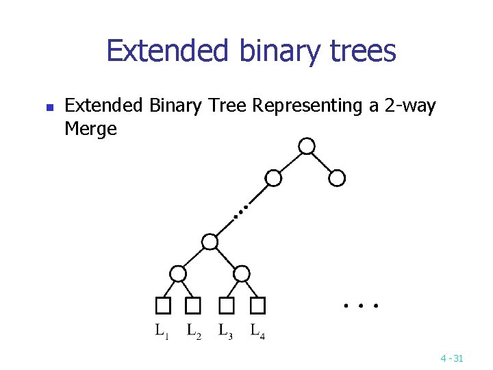
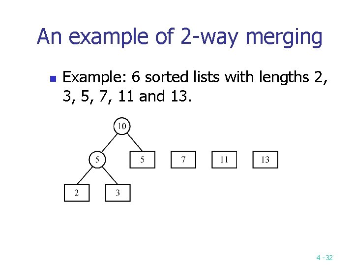
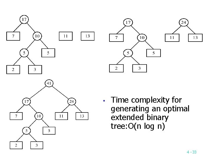
An example of 2 -way merging n Example: 6 sorted lists with lengths 2, 3, 5, 7, 11 and 13. 4 -32

§ Time complexity for generating an optimal extended binary tree: O(n log n) 4 -33

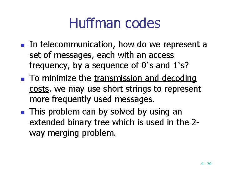
Huffman codes n n n In telecommunication, how do we represent a set of messages, each with an access frequency, by a sequence of 0’s and 1’s? To minimize the transmission and decoding costs, we may use short strings to represent more frequently used messages. This problem can by solved by using an extended binary tree which is used in the 2 way merging problem. 4 -34

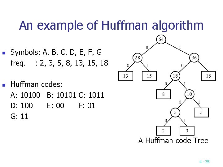
An example of Huffman algorithm n n Symbols: A, B, C, D, E, F, G freq. : 2, 3, 5, 8, 13, 15, 18 Huffman codes: A: 10100 B: 10101 C: 1011 D: 100 E: 00 F: 01 G: 11 A Huffman code Tree 4 -35

Chapter 4 Greedy method Input(A[1…n]) Solution ←ψ for i ← 1 to n do X ← SELECT(A) (最好有一data structure，經preprocessing後可以很快的找到( 包括delete)) If FEASIBLE( solution, x) then solution ← UNION( select, x) endif repeat Output (solution) 特點 (1)做一串decision (2)每個decision只關心自己是不是optimal一部份與其它無關 (可以local check) Note (1) Local optimal 須是global optimal (2)有時裡面隱含一個sorting 4 -36

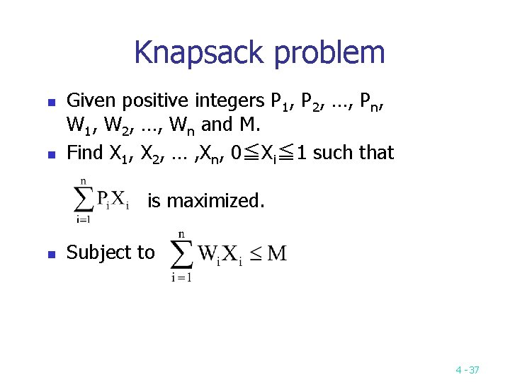
Knapsack problem n n Given positive integers P 1, P 2, …, Pn, W 1, W 2, …, Wn and M. Find X 1, X 2, … , Xn, 0≦Xi≦ 1 such that is maximized. n Subject to 4 -37

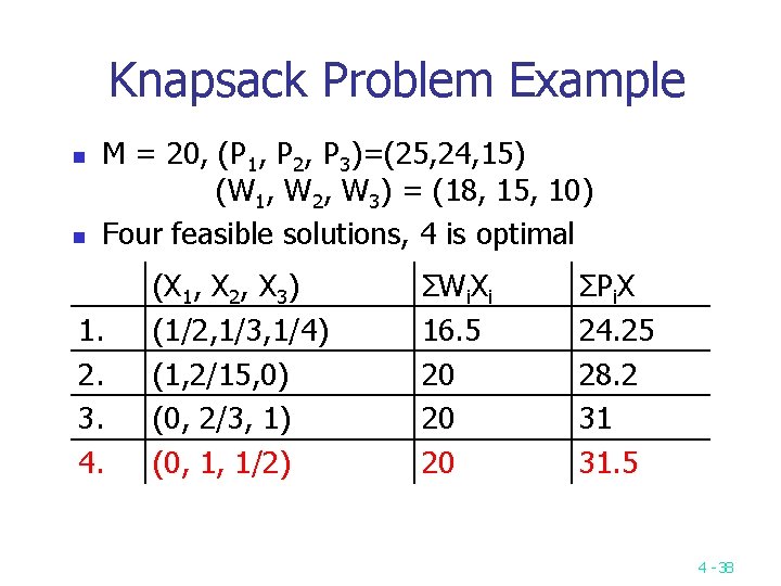
Knapsack Problem Example n n M = 20, (P 1, P 2, P 3)=(25, 24, 15) (W 1, W 2, W 3) = (18, 15, 10) Four feasible solutions, 4 is optimal 1. 2. 3. 4. (X 1, X 2, X 3) (1/2, 1/3, 1/4) (1, 2/15, 0) (0, 2/3, 1) (0, 1, 1/2) ΣWi. Xi 16. 5 20 20 20 ΣPi. X 24. 25 28. 2 31 31. 5 4 -38

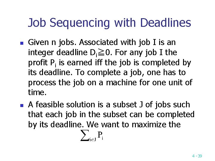
Job Sequencing with Deadlines n n Given n jobs. Associated with job I is an integer deadline Di≧ 0. For any job I the profit Pi is earned iff the job is completed by its deadline. To complete a job, one has to process the job on a machine for one unit of time. A feasible solution is a subset J of jobs such that each job in the subset can be completed by its deadline. We want to maximize the 4 -39

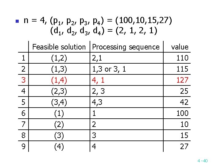
n n = 4, (p 1, p 2, p 3, p 4) = (100, 15, 27) (d 1, d 2, d 3, d 4) = (2, 1, 2, 1) Feasible solution 1 (1, 2) 2 (1, 3) 3 (1, 4) Processing sequence 2, 1 1, 3 or 3, 1 4 5 6 7 8 9 2, 3 4, 3 1 2 3 4 (2, 3) (3, 4) (1) (2) (3) (4) value 110 115 127 25 42 100 10 15 27 4 -40

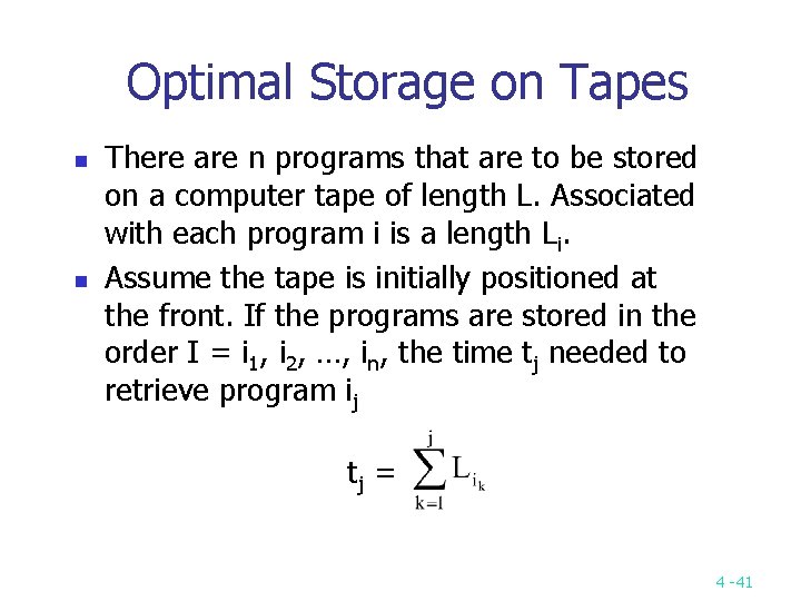
Optimal Storage on Tapes n n There are n programs that are to be stored on a computer tape of length L. Associated with each program i is a length Li. Assume the tape is initially positioned at the front. If the programs are stored in the order I = i 1, i 2, …, in, the time tj needed to retrieve program ij tj = 4 -41

Optimal Storage on Tapes n n If all programs are retrieved equally often, then the mean retrieval time (MRT) = This problem fits the ordering paradigm. Minimizing the MRT is equivalent to minimizing d(I) = 4 -42

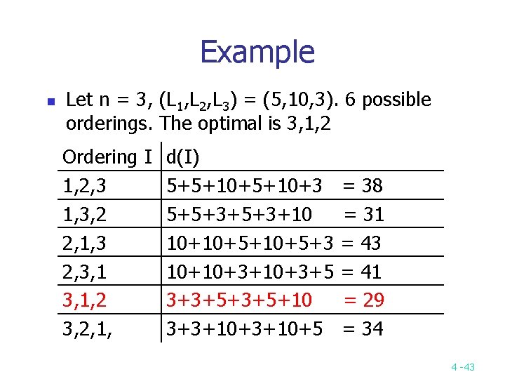
Example n Let n = 3, (L 1, L 2, L 3) = (5, 10, 3). 6 possible orderings. The optimal is 3, 1, 2 Ordering I d(I) 1, 2, 3 5+5+10+3 = 38 1, 3, 2 5+5+3+10 = 31 2, 1, 3 10+10+5+3 = 43 2, 3, 1 10+10+3+5 = 41 3, 1, 2 3+3+5+10 = 29 3, 2, 1, 3+3+10+5 = 34 4 -43