CHAPTER 3 SIMPLEX METHOD REGULAR SIMPLEX METHOD BY

CHAPTER #3 SIMPLEX METHOD ( REGULAR SIMPLEX METHOD) BY : FATIMAH AL-HAFIZ. Bisha University Information Systems Department 341 -NAL

Outlines • Introduction. • Standard Form of LP Model. • Simplex Method. • Algorithm. • Example. • Summary. OPERATIONS RESEARCH 2

Introduction • We saw how to solve tow-variables linear programming problems graphically. • Unfortunately, most of real-life LPs have many variables, so a method is needed to solve LPs with more than two variables. • We devote most of this chapter to discussion of the simplex algorithm which is used to solve even very large LPs. • In many industrial application, the simplex algorithm is used to solve LPs with thousands of constraints and variables. • In this chapter, we explain how the simplex method can be used to find optimal solutions to LPs. OPERATIONS RESEARCH 3

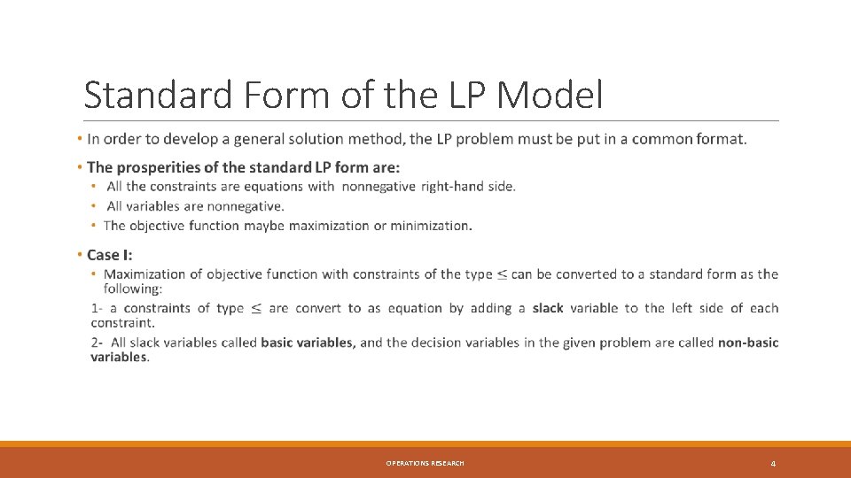
Standard Form of the LP Model OPERATIONS RESEARCH 4

Standard Form of the LP Model (cont. ) 3 - Objective function is converted to standard from by assign both sides to negative sign. Then, Case I is solving by using regular simplex method. OPERATIONS RESEARCH 5

Simplex Method • Simplex method : q Simplex method employs an iterative process that start at a feasible corner point, normally the origin and systematically moves from one feasible extreme point to another until the optimum point is eventually reached. q Simplex algorithm starts at the origin (0, 0) , which is usually referred to as the starting solution. It then moves to an adjacent corner point. q There are two rules that govern the selection of the next extreme point in the simplex method: § The next corner point must be adjacent to the current one. § The solution can never go back to a previously considered extreme point. OPERATIONS RESEARCH 6

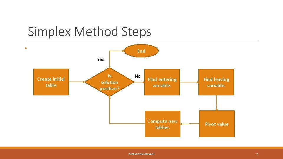
Simplex Method Steps • End Yes Create initial table Is solution positive? No Find entering variable. Find leaving variable. Compute new tablue. Pivot value OPERATIONS RESEARCH 7

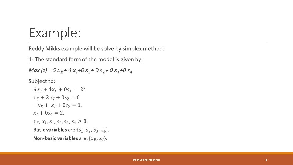
Example: OPERATIONS RESEARCH 8

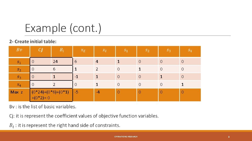
Example (cont. ) Max z 0 24 6 4 1 0 0 6 1 2 0 1 0 0 0 1 -1 1 0 0 2 0 1 0 0 0 1 -5 -4 0 0 (0*24)+(0*6)+(0*1) +(0*2)= 0 OPERATIONS RESEARCH 9

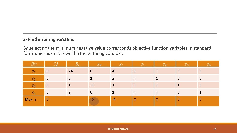
2 - Find entering variable. By selecting the minimum negative value corresponds objective function variables in standard form which is -5. It is will be the entering variable. Max z 0 24 6 4 1 0 0 6 1 2 0 1 0 0 0 1 -1 1 0 0 2 0 1 0 0 0 1 -5 -4 0 0 0 OPERATIONS RESEARCH 10

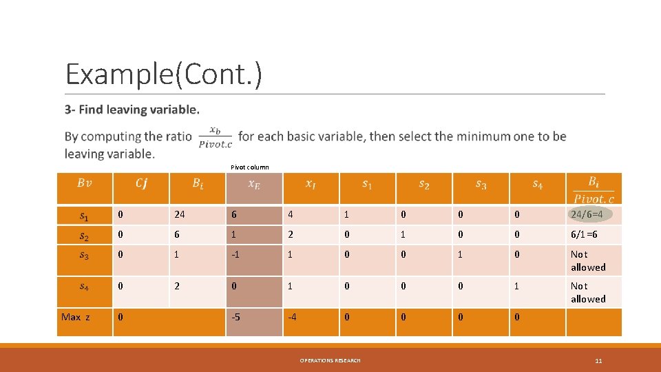
Example(Cont. ) Pivot column Max z 0 24 6 4 1 0 0 0 24/6=4 0 6 1 2 0 1 0 0 6/1=6 0 1 -1 1 0 0 1 0 Not allowed 0 2 0 1 0 0 0 1 Not allowed -5 -4 0 0 0 OPERATIONS RESEARCH 11

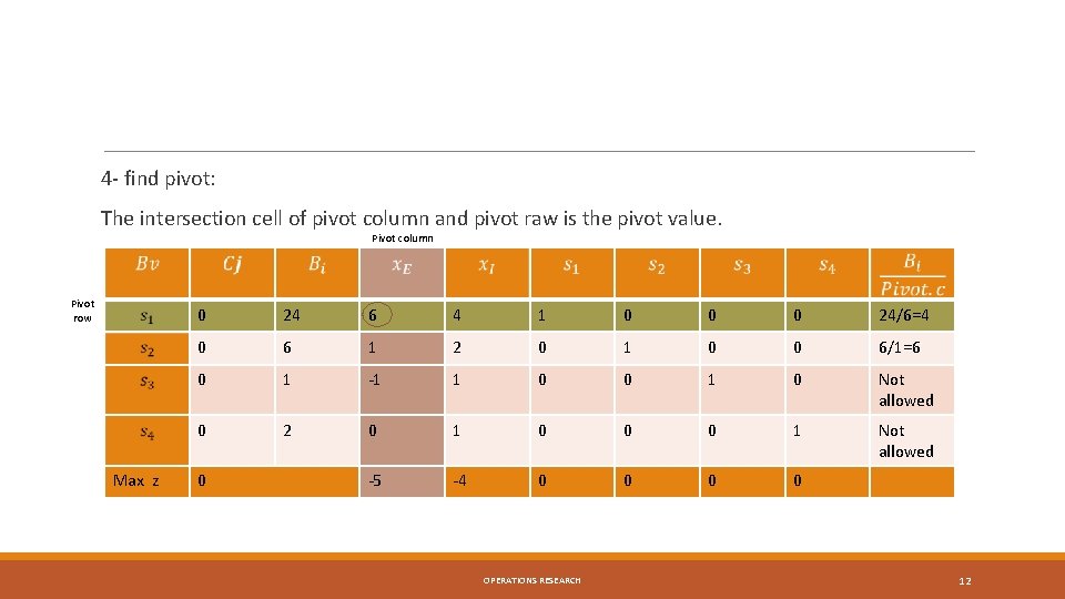
4 - find pivot: The intersection cell of pivot column and pivot raw is the pivot value. Pivot column Pivot row Max z 0 24 6 4 1 0 0 0 24/6=4 0 6 1 2 0 1 0 0 6/1=6 0 1 -1 1 0 0 1 0 Not allowed 0 2 0 1 0 0 0 1 Not allowed -5 -4 0 0 0 OPERATIONS RESEARCH 12

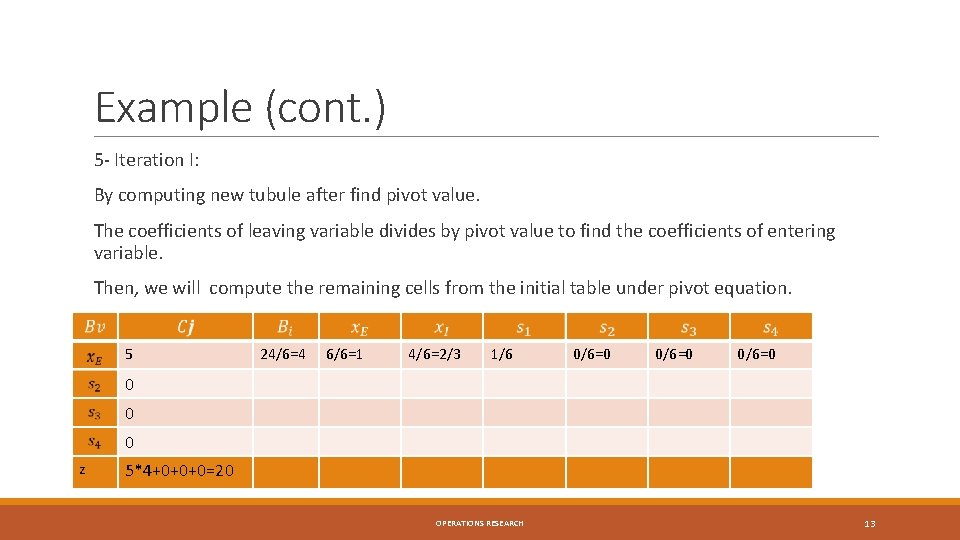
Example (cont. ) 5 - Iteration I: By computing new tubule after find pivot value. The coefficients of leaving variable divides by pivot value to find the coefficients of entering variable. Then, we will compute the remaining cells from the initial table under pivot equation. 5 24/6=4 6/6=1 4/6=2/3 1/6 0/6=0 0 z 5*4+0+0+0=20 OPERATIONS RESEARCH 13

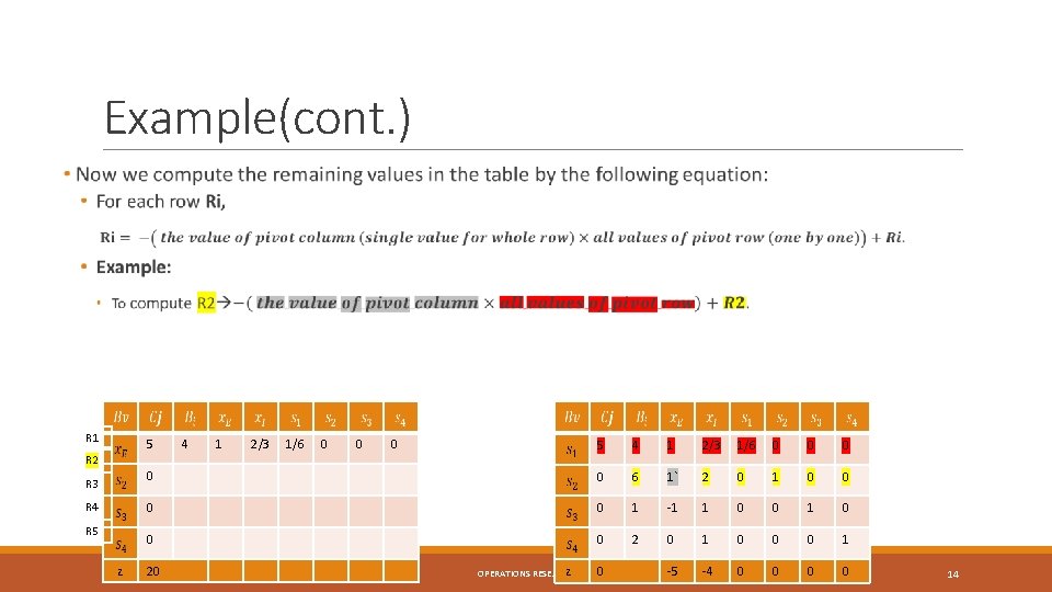
Example(cont. ) R 1 5 R 2 R 3 R 4 R 5 z 4 1 2/3 1/6 0 0 0 5 4 1 2/3 1/6 0 0 0 6 1` 2 0 1 0 0 1 -1 1 0 0 0 2 0 1 0 0 0 1 -5 -4 0 0 20 z OPERATIONS RESEARCH 0 14

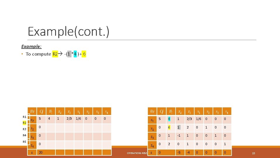
Example(cont. ) Example: • To compute R 2 -(1 *4 )+ 6 R 1 5 R 2 R 3 R 4 R 5 z 4 1 2/3 1/6 0 0 0 5 4 1 2/3 1/6 0 0 0 6 1 2 0 1 0 0 1 -1 1 0 0 0 2 0 1 0 0 0 1 -5 -4 0 0 20 z OPERATIONS RESEARCH 0 15

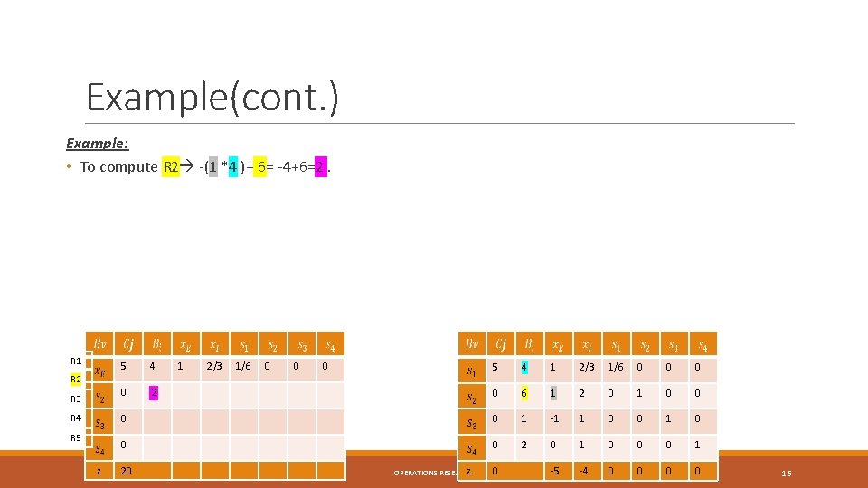
Example(cont. ) Example: • To compute R 2 -(1 *4 )+ 6= -4+6=2. R 1 R 2 R 3 R 4 R 5 z 5 4 0 2 1 2/3 1/6 0 0 0 5 4 1 2/3 1/6 0 0 6 1 2 0 1 0 0 1 -1 1 0 0 0 2 0 1 0 0 0 1 -5 -4 0 0 20 z OPERATIONS RESEARCH 0 16

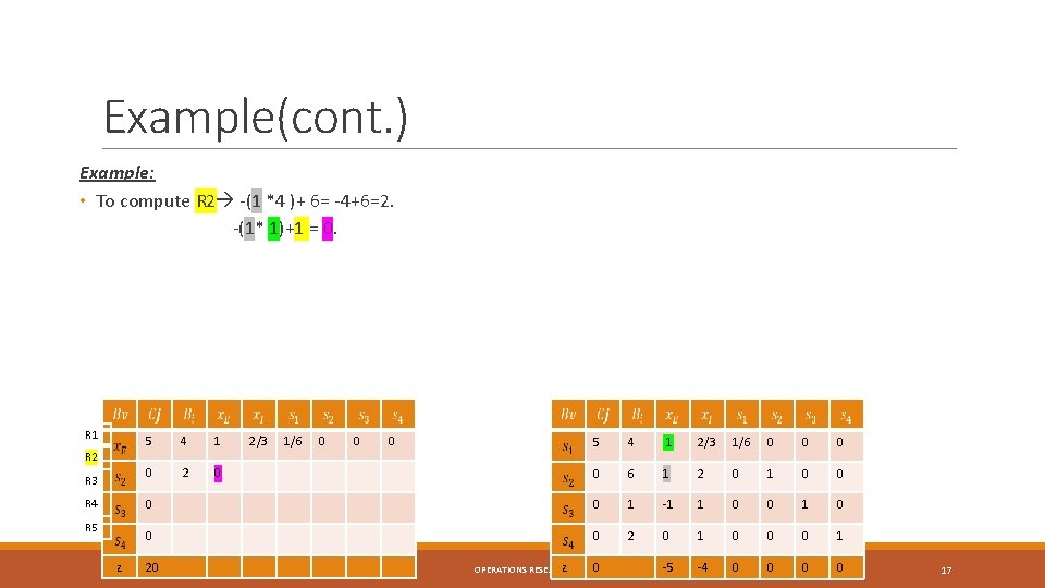
Example(cont. ) Example: • To compute R 2 -(1 *4 )+ 6= -4+6=2. -(1* 1)+1 = 0. R 1 R 2 R 3 R 4 R 5 z 5 4 1 0 2/3 1/6 0 0 0 5 4 1 2/3 1/6 0 0 6 1 2 0 1 0 0 1 -1 1 0 0 0 2 0 1 0 0 0 1 -5 -4 0 0 20 z OPERATIONS RESEARCH 0 17

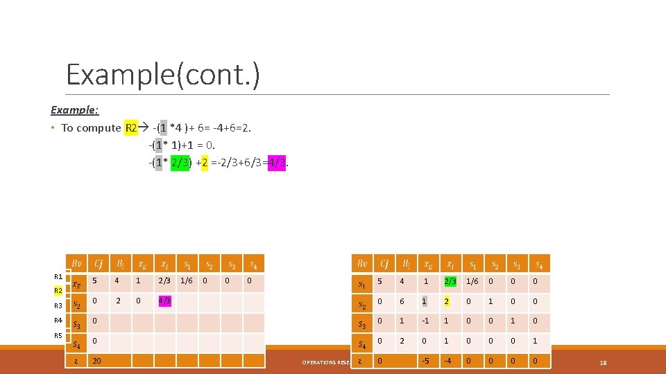
Example(cont. ) Example: • To compute R 2 -(1 *4 )+ 6= -4+6=2. -(1* 1)+1 = 0. -(1* 2/3) +2 =-2/3+6/3=4/3. R 1 R 2 R 3 R 4 R 5 z 5 4 1 2/3 0 2 0 4/3 1/6 0 0 0 5 4 1 2/3 1/6 0 0 6 1 2 0 1 0 0 1 -1 1 0 0 0 2 0 1 0 0 0 1 -5 -4 0 0 20 z OPERATIONS RESEARCH 0 18

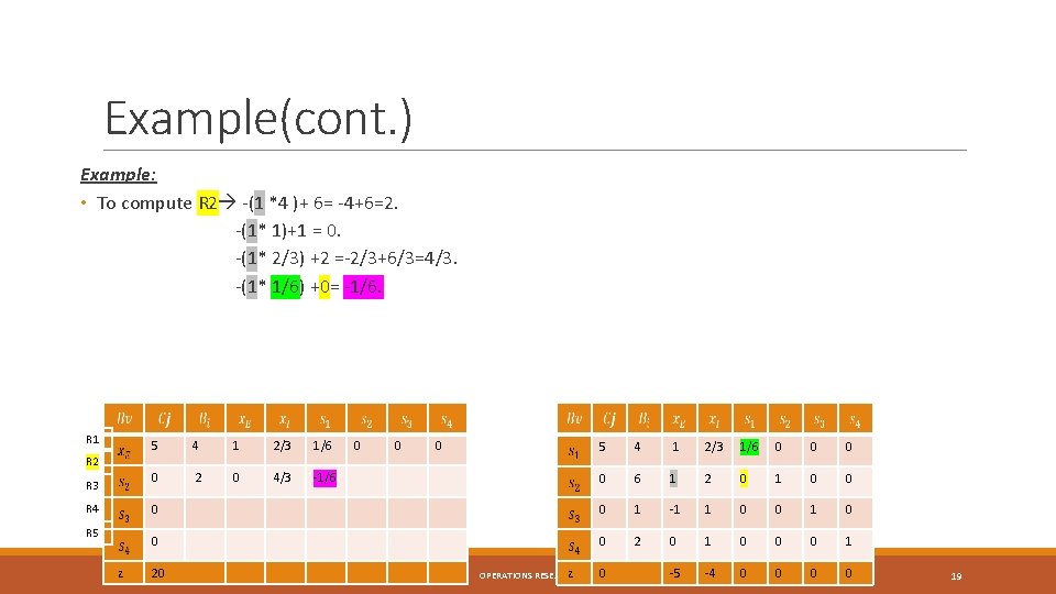
Example(cont. ) Example: • To compute R 2 -(1 *4 )+ 6= -4+6=2. -(1* 1)+1 = 0. -(1* 2/3) +2 =-2/3+6/3=4/3. -(1* 1/6) +0= -1/6. R 1 R 2 R 3 R 4 R 5 z 5 4 1 2/3 1/6 0 2 0 4/3 -1/6 0 0 0 5 4 1 2/3 1/6 0 0 6 1 2 0 1 0 0 1 -1 1 0 0 0 2 0 1 0 0 0 1 -5 -4 0 0 20 z OPERATIONS RESEARCH 0 19

Example(cont. ) Example: • To compute R 2 -(1 *4 )+ 6= -4+6=2. -(1* 1)+1 = 0. -(1* 2/3) +2 =-2/3+6/3=4/3. -(1* 1/6) +0= -1/6. -(1* 0) + 1= 1 R 2 R 3 R 4 R 5 z 5 4 1 2/3 1/6 0 0 2 0 4/3 -1/6 1 0 0 5 4 1 2/3 1/6 0 0 6 1 2 0 1 0 0 1 -1 1 0 0 0 2 0 1 0 0 0 1 -5 -4 0 0 20 z OPERATIONS RESEARCH 0 20

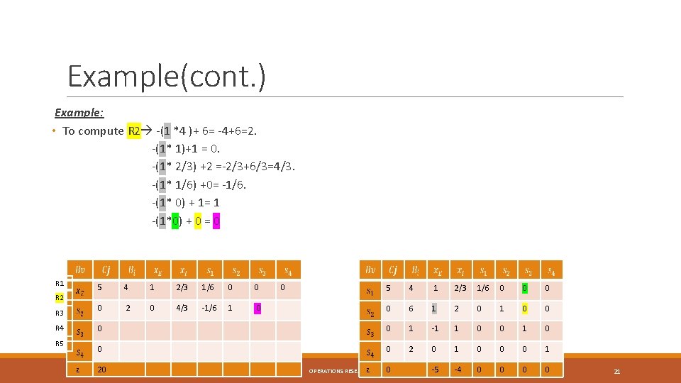
Example(cont. ) Example: • To compute R 2 -(1 *4 )+ 6= -4+6=2. -(1* 1)+1 = 0. -(1* 2/3) +2 =-2/3+6/3=4/3. -(1* 1/6) +0= -1/6. -(1* 0) + 1= 1 -(1*0) + 0 = 0 R 1 R 2 R 3 R 4 R 5 z 5 4 1 2/3 1/6 0 0 0 2 0 4/3 -1/6 1 0 0 5 4 1 2/3 1/6 0 0 6 1 2 0 1 0 0 1 -1 1 0 0 0 2 0 1 0 0 0 1 -5 -4 0 0 20 z OPERATIONS RESEARCH 0 21

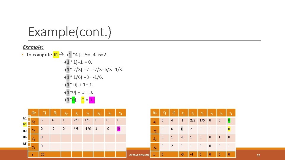
Example(cont. ) Example: • To compute R 2 -(1 *4 )+ 6= -4+6=2. -(1* 1)+1 = 0. -(1* 2/3) +2 =-2/3+6/3=4/3. -(1* 1/6) +0= -1/6. -(1* 0) + 1= 1. -(1*0) + 0 = 0. R 1 R 2 R 3 R 4 R 5 z 5 4 1 2/3 1/6 0 0 0 0 2 0 4/3 -1/6 1 0 0 0 6 1 2 0 1 0 0 1 -1 1 0 0 0 2 0 1 0 0 0 1 -5 -4 0 0 20 z OPERATIONS RESEARCH 0 22

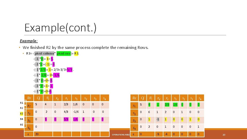
Example(cont. ) Example: • We finished R 2 by the same process complete the remaining Rows. • R 3= -(pivot column* pivot row)+ R 3. -(-1 *4)+ 1= 5. -(-1*1)+(-1)= 0. -(-1*2/3)+ 1= 2/3+3/3=5/3. -(-1* 1/6)+ 0= 1/6. -(-1* 0)+0= 0. -(-1* 0)+1= 1. -(-1* 0)+0=0. R 1 R 2 R 3 R 4 R 5 5 4 1 2/3 1/6 0 0 0 0 2 0 4/3 -1/6 1 0 0 0 6 1 2 0 1 0 0 0 5/3 1/6 0 1 0 0 1 -1 1 0 0 2 0 1 0 0 0 1 -5 -4 0 0 0 z 20 z OPERATIONS RESEARCH 0 23

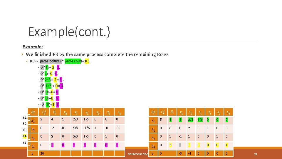
Example(cont. ) Example: • We finished R 3 by the same process complete the remaining Rows. • R 3= -(pivot column* pivot row)+ R 3. -(0 *4)+ 2= 2. -(0*1)+0= 0. -(0*2/3)+ 1= 1. -(0* 1/6)+ 0= 0. -(0* 0)+0= 0. -(-0* 0)+1=1. R 1 R 2 R 3 R 4 R 5 z 5 4 1 2/3 1/6 0 0 0 0 2 0 4/3 -1/6 1 0 0 0 6 1 2 0 1 0 0 0 5/3 1/6 0 1 0 0 1 -1 1 0 0 2 0 1 0 0 0 1 -5 -4 0 0 20 z OPERATIONS RESEARCH 0 24

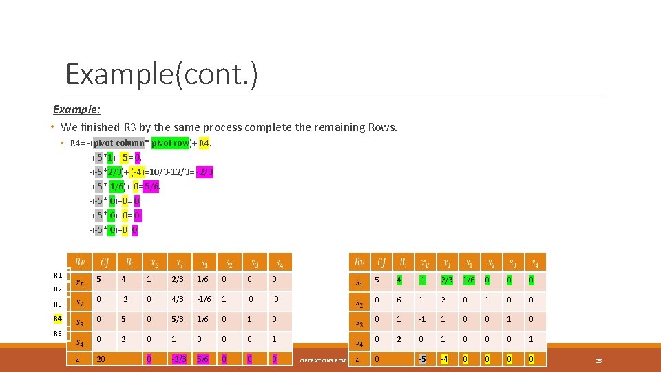
Example(cont. ) Example: • We finished R 3 by the same process complete the remaining Rows. • R 4= -(pivot column* pivot row)+ R 4. -(-5*1)+-5= 0. -(-5*2/3)+ (-4)=10/3 -12/3= -2/3. -(-5* 1/6)+ 0= 5/6. -(-5* 0)+0= 0. -(-5* 0)+0=0. R 1 R 2 R 3 R 4 R 5 z 5 4 1 2/3 1/6 0 0 0 0 2 0 4/3 -1/6 1 0 0 0 6 1 2 0 1 0 0 0 5/3 1/6 0 1 0 0 1 -1 1 0 0 2 0 1 0 0 0 1 0 -2/3 5/6 0 0 0 -5 -4 0 0 20 z OPERATIONS RESEARCH 0 25

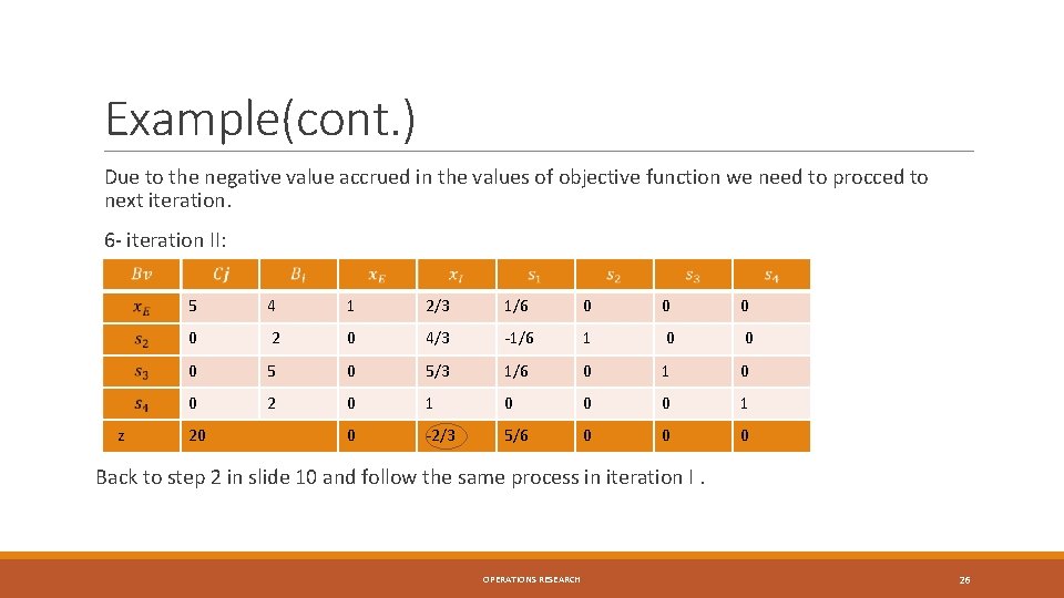
Example(cont. ) Due to the negative value accrued in the values of objective function we need to procced to next iteration. 6 - iteration II: z 5 4 1 2/3 1/6 0 0 2 0 4/3 -1/6 1 0 0 0 5/3 1/6 0 1 0 0 2 0 1 0 0 0 1 0 -2/3 5/6 0 0 0 20 Back to step 2 in slide 10 and follow the same process in iteration I. OPERATIONS RESEARCH 26

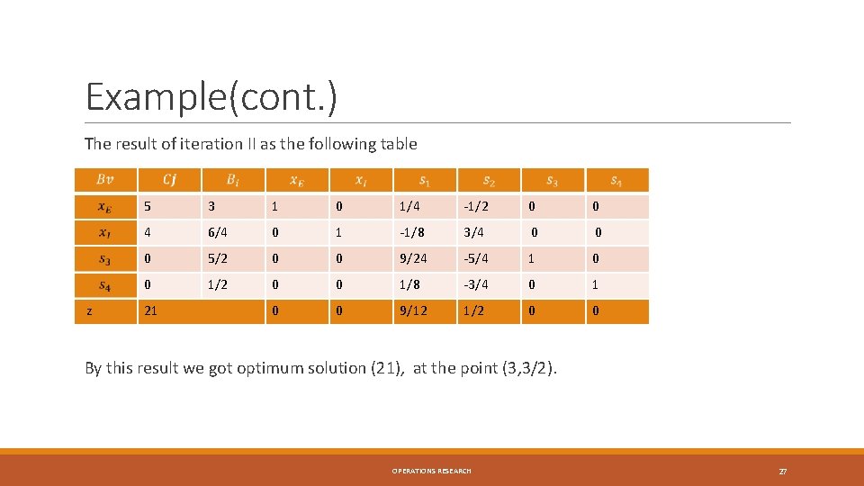
Example(cont. ) The result of iteration II as the following table z 5 3 1 0 1/4 -1/2 0 0 4 6/4 0 1 -1/8 3/4 0 0 0 5/2 0 0 9/24 -5/4 1 0 0 1/2 0 0 1/8 -3/4 0 1 0 0 9/12 1/2 0 0 21 By this result we got optimum solution (21), at the point (3, 3/2). OPERATIONS RESEARCH 27

Summery OPERATIONS RESEARCH 28