Chapter 3 Selected Basic Concepts in Statistics Part
Chapter 3 Selected Basic Concepts in Statistics, Part 1 Expected Value, Variance, Standard Deviation n Numerical summaries of selected statistics n Sampling distributions n
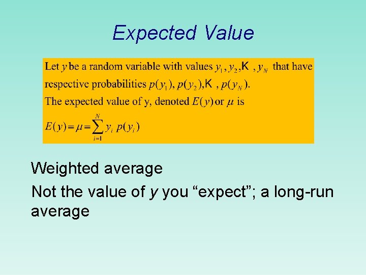
Expected Value Weighted average Not the value of y you “expect”; a long-run average
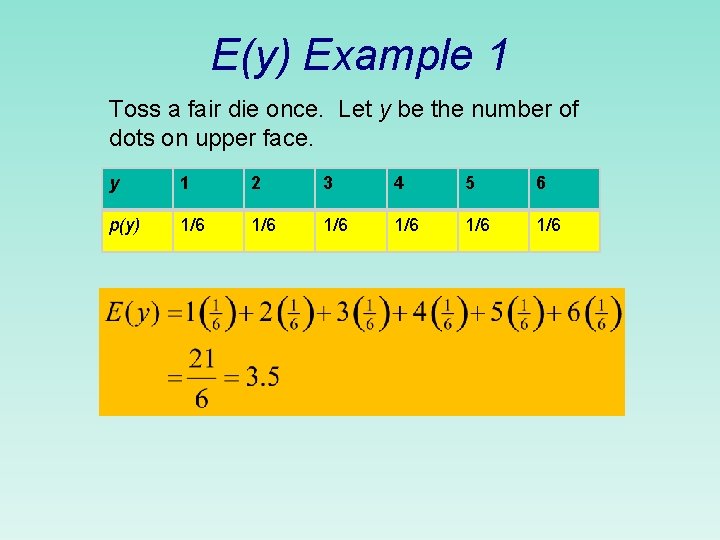
E(y) Example 1 Toss a fair die once. Let y be the number of dots on upper face. y 1 2 3 4 5 6 p(y) 1/6 1/6 1/6
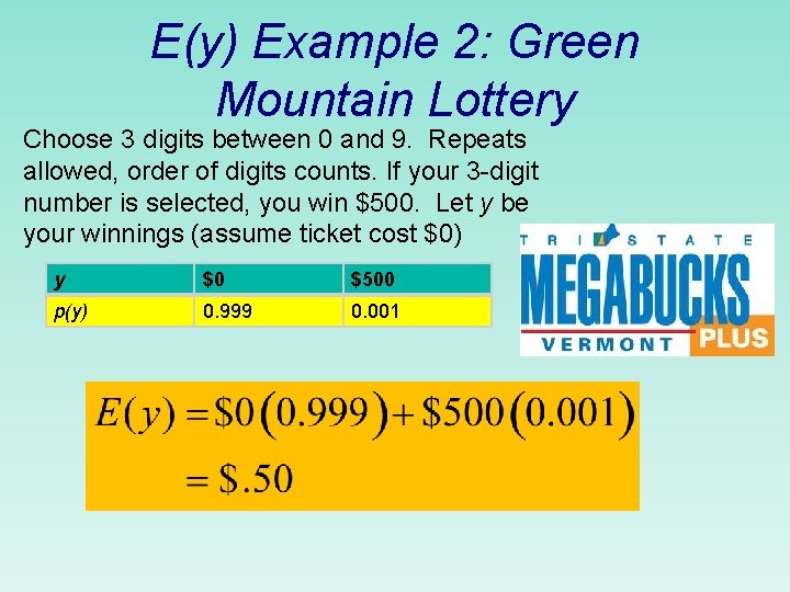
E(y) Example 2: Green Mountain Lottery Choose 3 digits between 0 and 9. Repeats allowed, order of digits counts. If your 3 -digit number is selected, you win $500. Let y be your winnings (assume ticket cost $0) y $0 $500 p(y) 0. 999 0. 001

n n US Roulette Wheel and Table The roulette wheel has alternating black and red slots numbered 1 through 36. There also 2 green slots numbered 0 and 00. A bet on any one of the 38 numbers (1 -36, 0, or 00) pays odds of 35: 1; that is. . . If you bet $1 on the winning number, you receive $36, so your winnings are $35 American Roulette 0 - 00 (The European version has only one 0. )

US Roulette Wheel: Expected Value of a $1 bet on a single number n Let y be your winnings resulting from a $1 bet on a single number; y has 2 possible values y p(y) n n n -1 37/38 35 1/38 E(y)= -1(37/38)+35(1/38)= -. 05 So on average the house wins 5 cents on every such bet. A “fair” game would have E(y)=0. The roulette wheels are spinning 24/7, winning big $$ for the house, resulting in …

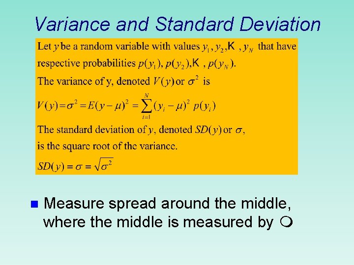
Variance and Standard Deviation n Measure spread around the middle, where the middle is measured by
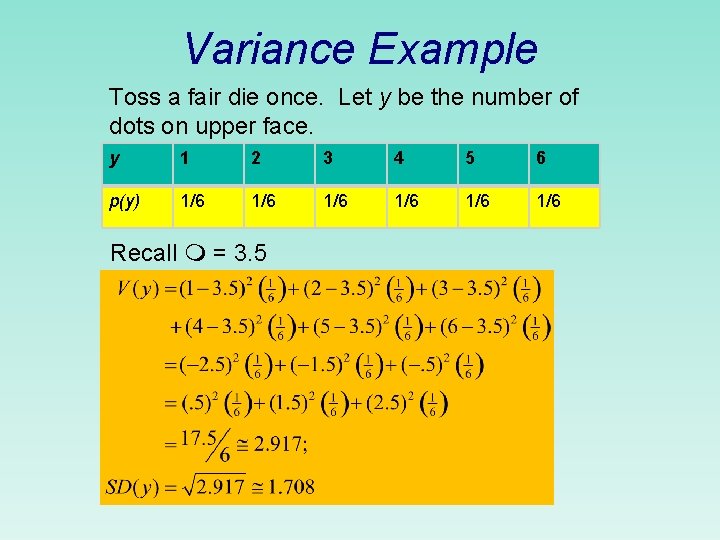
Variance Example Toss a fair die once. Let y be the number of dots on upper face. y 1 2 3 4 5 6 p(y) 1/6 1/6 1/6 Recall = 3. 5
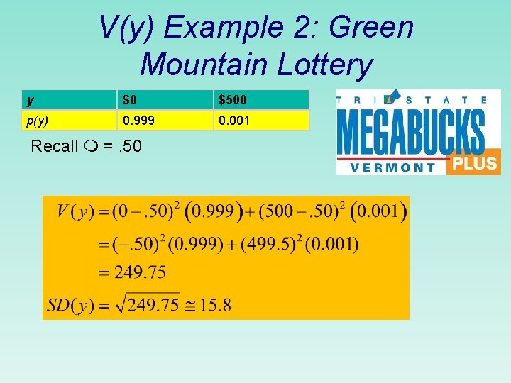
V(y) Example 2: Green Mountain Lottery y $0 $500 p(y) 0. 999 0. 001 Recall =. 50
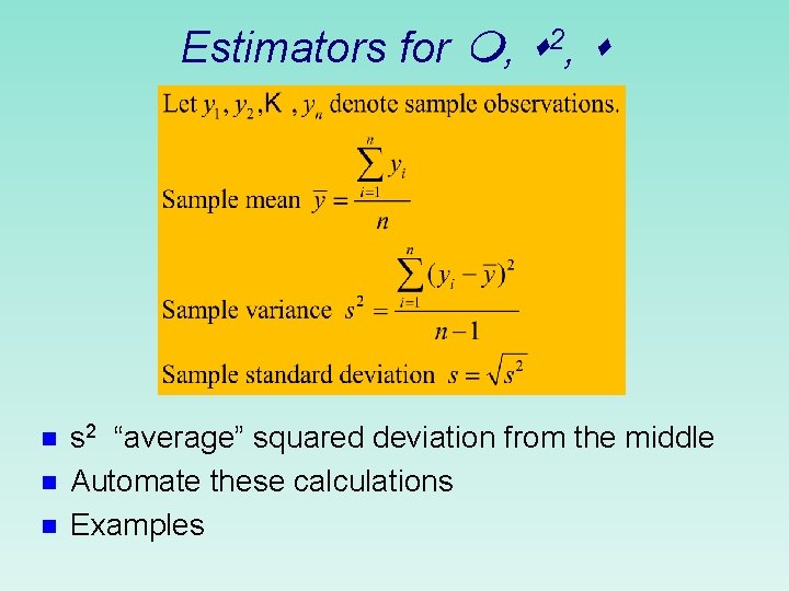
Estimators for , 2, n n n s 2 “average” squared deviation from the middle Automate these calculations Examples
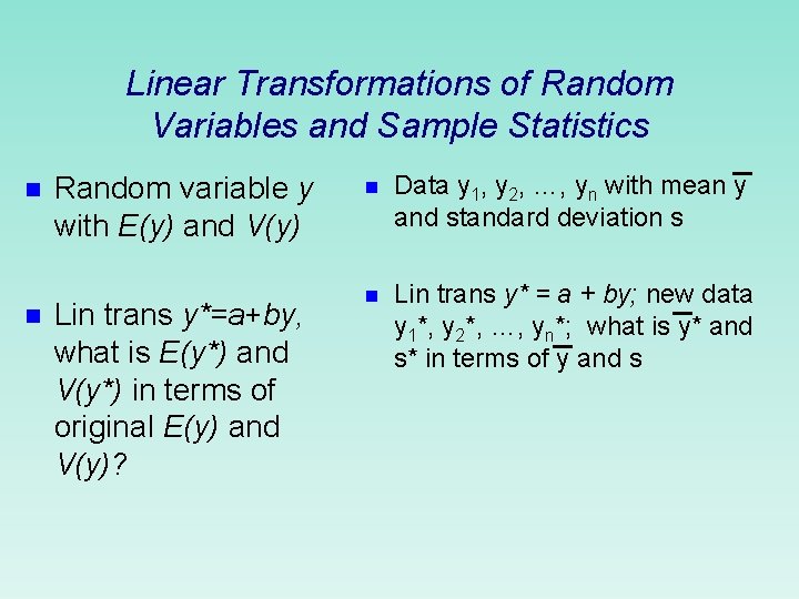
Linear Transformations of Random Variables and Sample Statistics n n Random variable y with E(y) and V(y) Lin trans y*=a+by, what is E(y*) and V(y*) in terms of original E(y) and V(y)? n Data y 1, y 2, …, yn with mean y and standard deviation s n Lin trans y* = a + by; new data y 1*, y 2*, …, yn*; what is y* and s* in terms of y and s
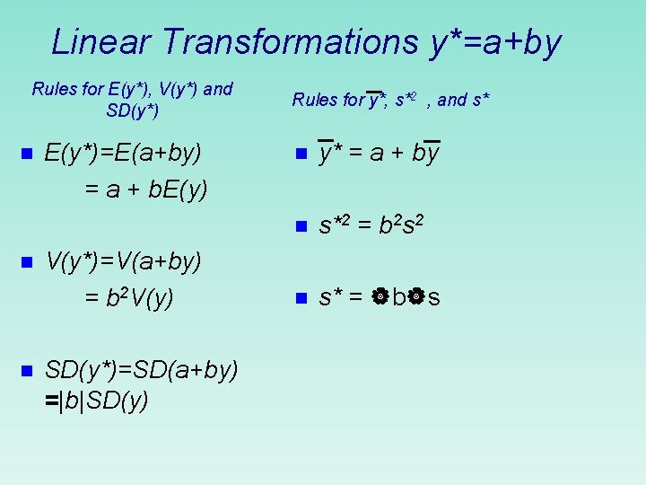
Linear Transformations y*=a+by Rules for E(y*), V(y*) and SD(y*) n n n E(y*)=E(a+by) = a + b. E(y) V(y*)=V(a+by) = b 2 V(y) SD(y*)=SD(a+by) =|b|SD(y) Rules for y*, s*2 , and s* n y* = a + by n s*2 = b 2 s 2 n s* = b s

Expected Value and Standard Deviation of Linear Transformation a + by Let y=number of repairs a new computer needs each year. Suppose E(y)= 0. 20 and SD(y)=0. 55 The service contract for the computer offers unlimited repairs for $100 per year plus a $25 service charge for each repair. What are the mean and standard deviation of the yearly cost of the service contract? Cost = $100 + $25 y E(cost) = E($100+$25 y)=$100+$25 E(y)=$100+$25*0. 20= = $100+$5=$105 SD(cost)=SD($100+$25 y)=SD($25 y)=$25*SD(y)=$25*0. 55= =$13. 75

Addition and Subtraction Rules for Random Variables n n n E(X+Y) = E(X) + E(Y); E(X-Y) = E(X) - E(Y) When X and Y are independent random variables: 1. Var(X+Y)=Var(X)+Var(Y) 2. SD(X+Y)= SD’s do not add: SD(X+Y)≠ SD(X)+SD(Y) 3. Var(X−Y)=Var(X)+Var(Y) 4. SD(X −Y)= SD’s do not subtract: SD(X−Y)≠ SD(X)−SD(Y) SD(X−Y)≠ SD(X)+SD(Y)
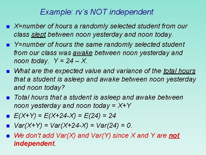
Example: rv’s NOT independent n n n n X=number of hours a randomly selected student from our class slept between noon yesterday and noon today. Y=number of hours the same randomly selected student from our class was awake between noon yesterday and noon today. Y = 24 – X. What are the expected value and variance of the total hours that a student is asleep and awake between noon yesterday and noon today? Total hours that a student is asleep and awake between noon yesterday and noon today = X+Y E(X+Y) = E(X+24 -X) = E(24) = 24 Var(X+Y) = Var(X+24 -X) = Var(24) = 0. We don't add Var(X) and Var(Y) since X and Y are not independent.
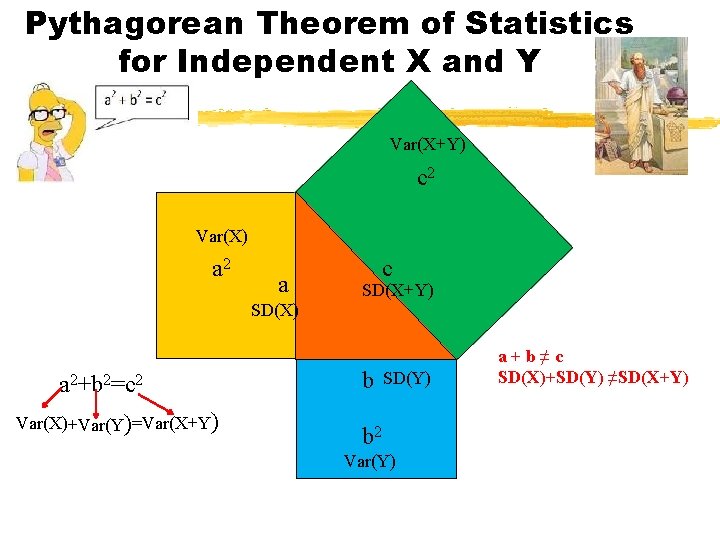
Pythagorean Theorem of Statistics for Independent X and Y Var(X+Y) c 2 Var(X) a 2 a c SD(X+Y) SD(X) a 2+b 2=c 2 Var(X)+Var(Y)=Var(X+Y) b SD(Y) b 2 Var(Y) a+b≠c SD(X)+SD(Y) ≠SD(X+Y)
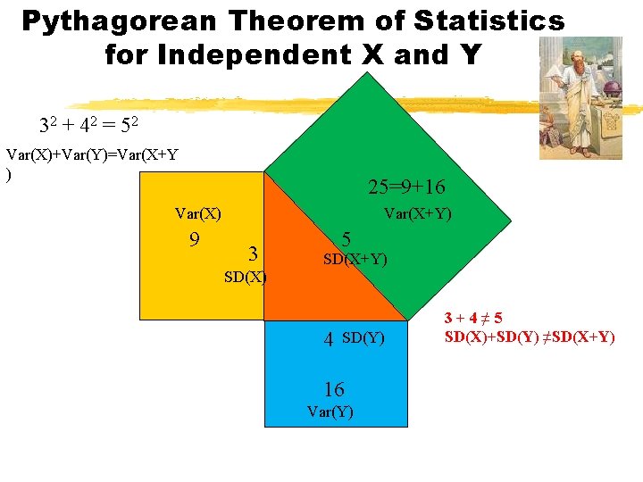
Pythagorean Theorem of Statistics for Independent X and Y 32 + 42 = 52 Var(X)+Var(Y)=Var(X+Y ) 25=9+16 Var(X) 9 Var(X+Y) 3 5 SD(X+Y) SD(X) 4 SD(Y) 16 Var(Y) 3+4≠ 5 SD(X)+SD(Y) ≠SD(X+Y)
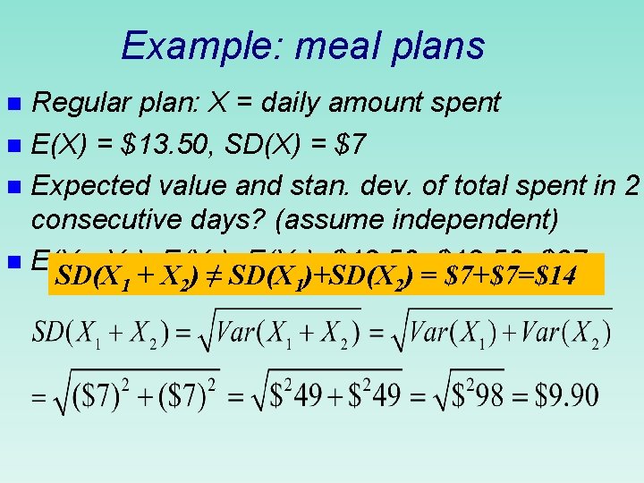
Example: meal plans Regular plan: X = daily amount spent n E(X) = $13. 50, SD(X) = $7 n Expected value and stan. dev. of total spent in 2 consecutive days? (assume independent) n E(X 1+X 2)=E(X 1)+E(X 2)=$13. 50+$13. 50=$27 SD(X + X ) ≠ SD(X )+SD(X ) = $7+$7=$14 n 1 2

Example: meal plans (cont. ) Jumbo plan for football players Y=daily amount spent n E(Y) = $24. 75, SD(Y) = $9. 50 n Amount by which football player’s spending exceeds regular student spending is Y-X n E(Y-X)=E(Y)–E(X)=$24. 75 -$13. 50=$11. 25 SD(Y X) ≠ SD(Y) SD(X) = $9. 50 n $7=$2. 50
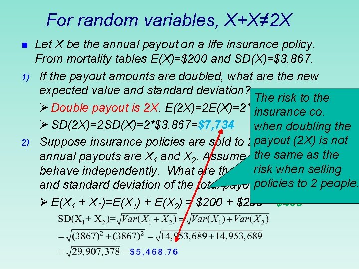
For random variables, X+X≠ 2 X n 1) 2) Let X be the annual payout on a life insurance policy. From mortality tables E(X)=$200 and SD(X)=$3, 867. If the payout amounts are doubled, what are the new expected value and standard deviation? The risk to the Ø Double payout is 2 X. E(2 X)=2 E(X)=2*$200=$400 insurance co. Ø SD(2 X)=2 SD(X)=2*$3, 867=$7, 734 when doubling the Suppose insurance policies are sold to 2 payout people. (2 X) Theis not the 2 same as the annual payouts are X 1 and X 2. Assume the people risk when selling behave independently. What are the expected value policies to 2 people. and standard deviation of the total payout? Ø E(X 1 + X 2)=E(X 1) + E(X 2) = $200 + $200 = $400
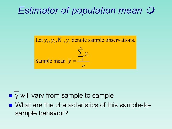
Estimator of population mean n n y will vary from sample to sample What are the characteristics of this sample-tosample behavior?
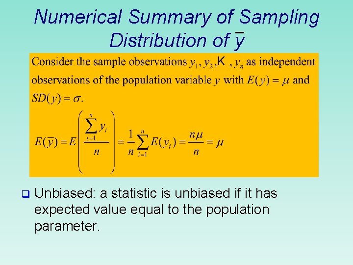
Numerical Summary of Sampling Distribution of y q Unbiased: a statistic is unbiased if it has expected value equal to the population parameter.
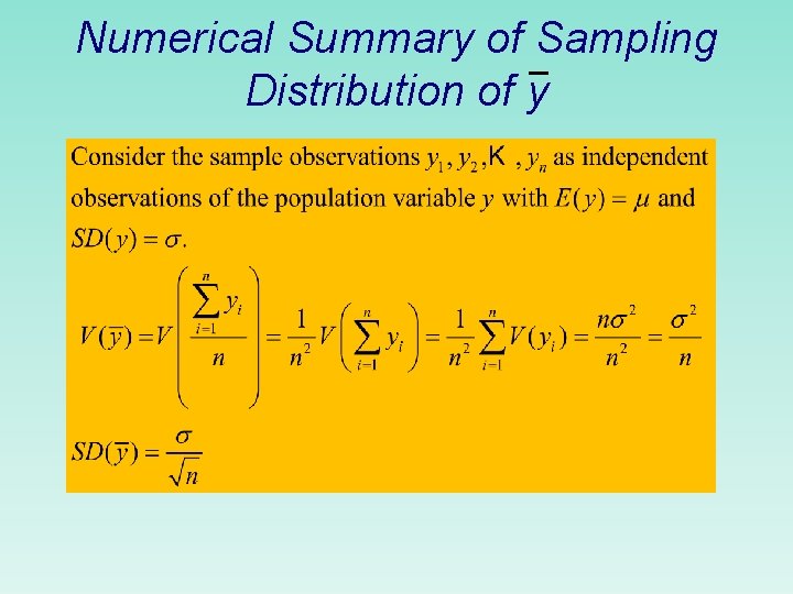
Numerical Summary of Sampling Distribution of y
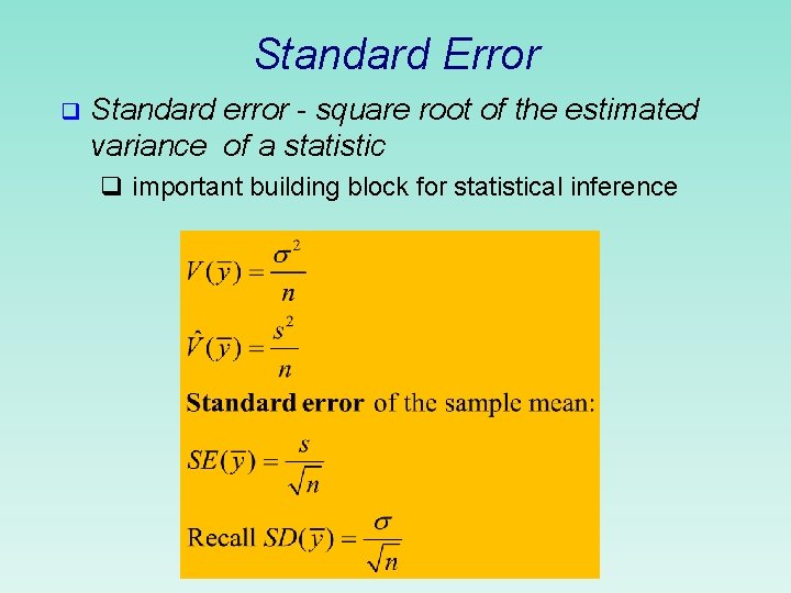
Standard Error q Standard error - square root of the estimated variance of a statistic q important building block for statistical inference
Shape? We have numerical summaries of the sampling distribution of y n What about the shape of the sampling distribution of y ? n
THE CENTRAL LIMIT THEOREM The World is Normal Theorem
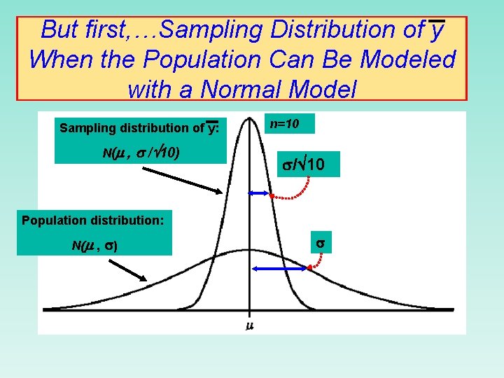
But first, …Sampling Distribution of y When the Population Can Be Modeled with a Normal Model Sampling distribution of y: N( , / 10) n=10 / 10 Population distribution: N( , )
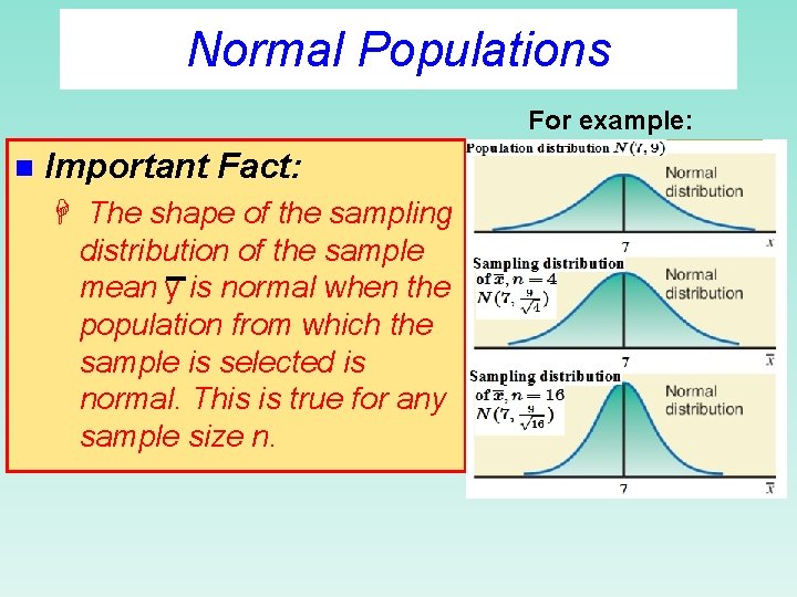
Normal Populations For example: n Important Fact: H The shape of the sampling distribution of the sample mean y is normal when the population from which the sample is selected is normal. This is true for any sample size n.
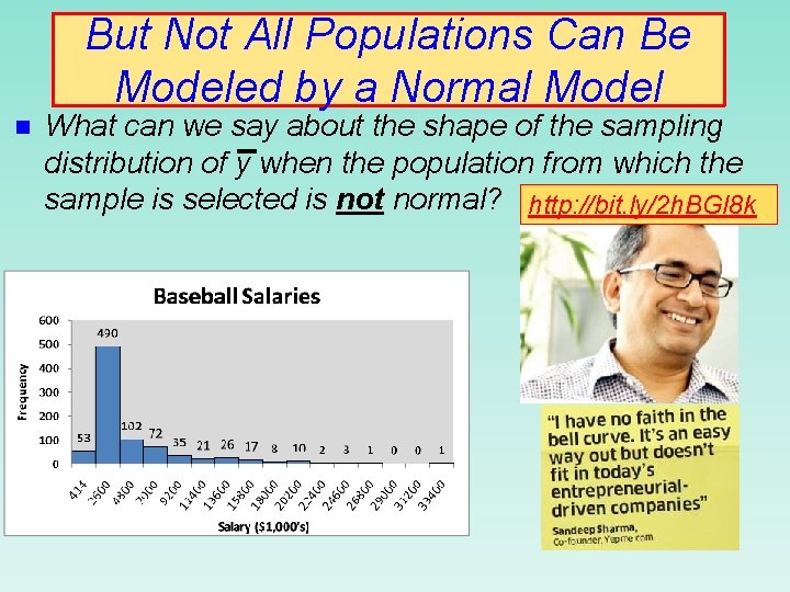
But Not All Populations Can Be Modeled by a Normal Model n What can we say about the shape of the sampling distribution of y when the population from which the sample is selected is not normal? http: //bit. ly/2 h. BGl 8 k
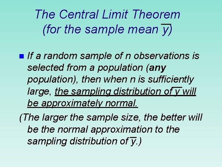
The Central Limit Theorem (for the sample mean y) If a random sample of n observations is selected from a population (any population), then when n is sufficiently large, the sampling distribution of y will be approximately normal. (The larger the sample size, the better will be the normal approximation to the sampling distribution of y. ) n
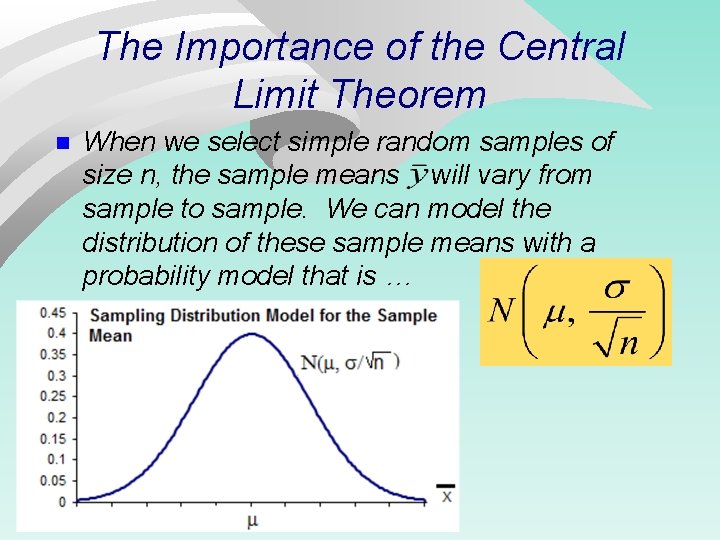
The Importance of the Central Limit Theorem n When we select simple random samples of size n, the sample means will vary from sample to sample. We can model the distribution of these sample means with a probability model that is …
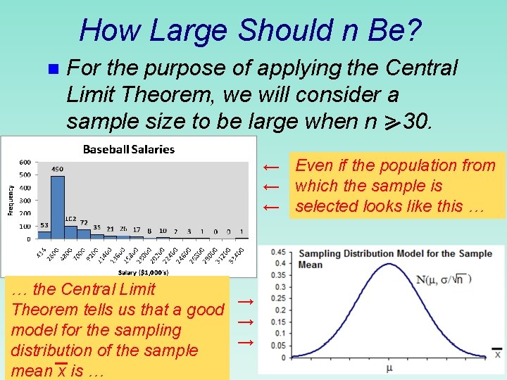
How Large Should n Be? n For the purpose of applying the Central Limit Theorem, we will consider a sample size to be large when n > 30. ← Even if the population from ← which the sample is ← selected looks like this … … the Central Limit → Theorem tells us that a good → model for the sampling → distribution of the sample mean x is …

Summary Population: mean ; stand dev. ; shape of population dist. is unknown; value of is unknown; select random sample of size n; Sampling distribution of x: mean ; stand. dev. / n; always true! By the Central Limit Theorem: the shape of the sampling distribution is approx normal, that is x ~ N( , / n)

Too Heavy for the Elevator? Mean weight of US men is 190 lb, the standard deviation is 59 lb. A large freight elevator has a weight limit of 6600 lb. Find the probability that 30 men in the elevator will exceed the weight limit. 30 men over 6600 lb. ; so the mean weight of the 30 men must be greater than 6600/30 = 220 lb. • • Copyright © 2016, 2014, 2012, 2009 Pearson Education, Inc. 35
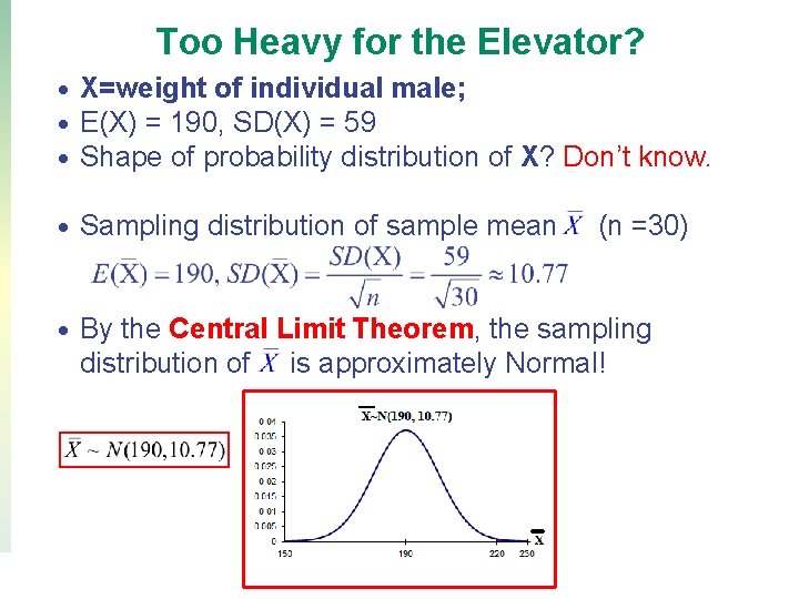
Too Heavy for the Elevator? • • • X=weight of individual male; E(X) = 190, SD(X) = 59 Shape of probability distribution of X? Don’t know. • Sampling distribution of sample mean • By the Central Limit Theorem, the sampling distribution of is approximately Normal! Copyright © 2016, 2014, 2012, 2009 Pearson Education, Inc. (n =30) 36
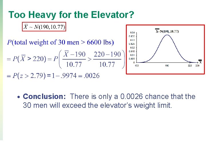
Too Heavy for the Elevator? • Conclusion: There is only a 0. 0026 chance that the 30 men will exceed the elevator’s weight limit. Copyright © 2016, 2014, 2012, 2009 Pearson Education, Inc. 37
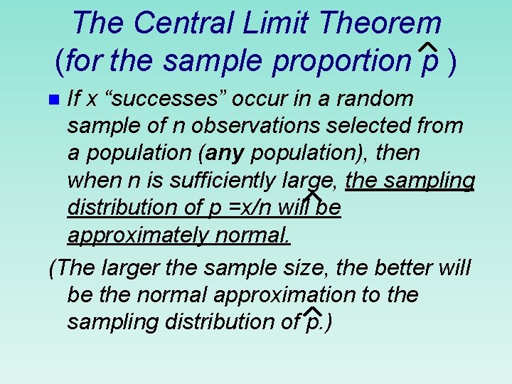
The Central Limit Theorem (for the sample proportion p ) If x “successes” occur in a random sample of n observations selected from a population (any population), then when n is sufficiently large, the sampling distribution of p =x/n will be approximately normal. (The larger the sample size, the better will be the normal approximation to the sampling distribution of p. ) n
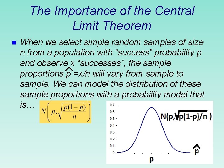
The Importance of the Central Limit Theorem n When we select simple random samples of size n from a population with “success” probability p and observe x “successes”, the sample proportions p =x/n will vary from sample to sample. We can model the distribution of these sample proportions with a probability model that is…
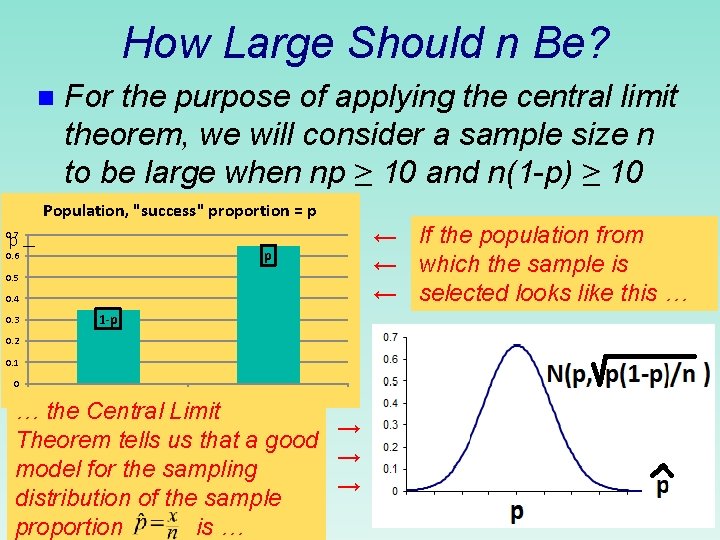
How Large Should n Be? n For the purpose of applying the central limit theorem, we will consider a sample size n to be large when np ≥ 10 and n(1 -p) ≥ 10 Population, "success" proportion = p 0. 7 p __ p 0. 6 0. 5 0. 4 0. 3 1 -p 0. 2 0. 1 0 0 1 … the Central Limit → Theorem tells us that a good → model for the sampling → distribution of the sample proportion is … ← If the population from ← which the sample is ← selected looks like this …

End of Chapter 3, part 1
- Slides: 41