Chapter 3 Roots of Equations Objectives Understanding what

Chapter 3 Roots of Equations
Objectives • Understanding what roots problems are and where they occur in engineering and science • Knowing how to determine a root graphically • Knowing how to solve a root problem with bracketing method • Understand the open method and recognize the difference between the open and bracketing methods • Knowing how to use MATLAB built-in function
Content • Introduction • Graphical method • Bracketing method (Bisection and false position) • Open method (Newton Raphson and secant methods) • MATLAB built-in function • Conclusion
Introduction Many engineering and science problems predict dependent variable(s) as a function of independent variables Heat balance : time&space Mass balance : mass concen. : time&space Kirchoff’s law: current/voltage : time
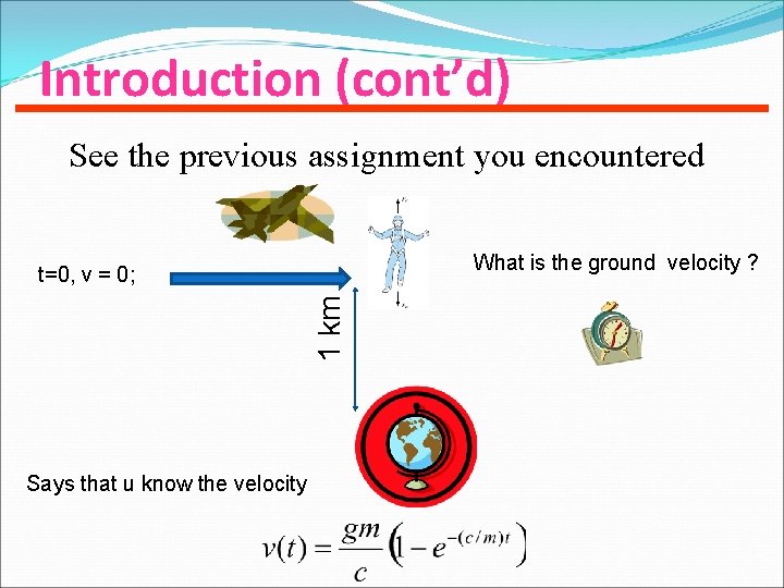
Introduction (cont’d) See the previous assignment you encountered What is the ground velocity ? 1 km t=0, v = 0; Says that u know the velocity
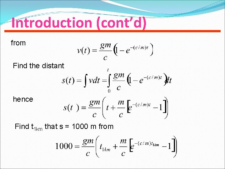
Introduction (cont’d) from Find the distant hence Find t 1 km that s = 1000 m from
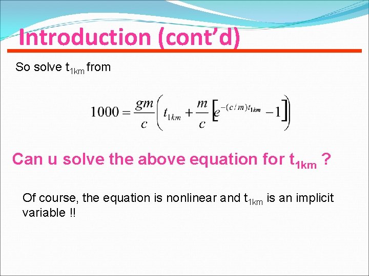
Introduction (cont’d) So solve t 1 km from Can u solve the above equation for t 1 km ? Of course, the equation is nonlinear and t 1 km is an implicit variable !!
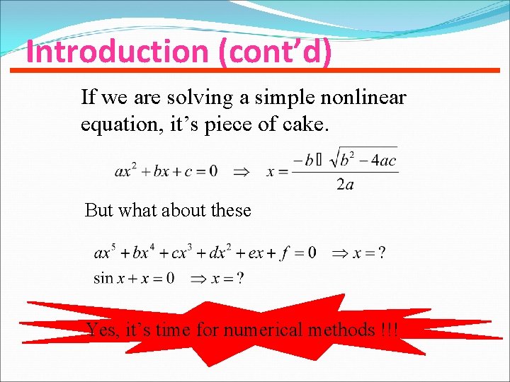
Introduction (cont’d) If we are solving a simple nonlinear equation, it’s piece of cake. But what about these Yes, it’s time for numerical methods !!!
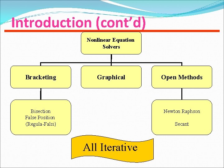
Introduction (cont’d) Nonlinear Equation Solvers Bracketing Graphical Bisection False Position (Regula-Falsi) Open Methods Newton Raphson Secant All Iterative
Graphical… Graphical method means that we plot graph from the target nonlinear equation and observe the zero of it !! Very simple but too iterative. Here try with parachutist problem…. .
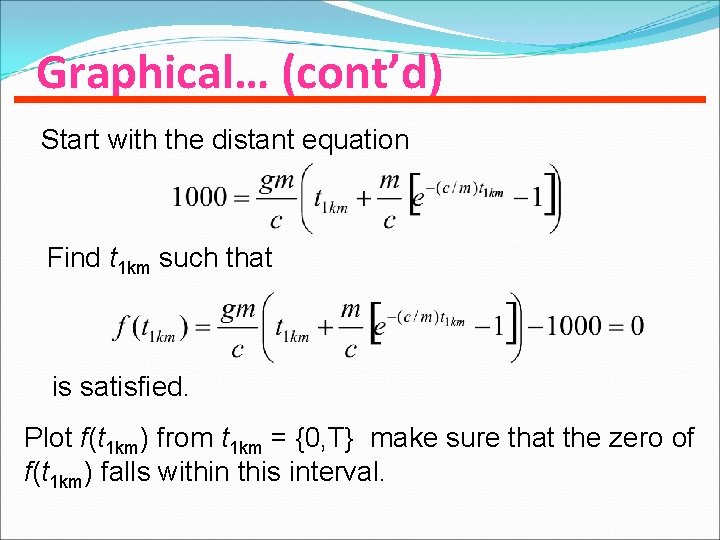
Graphical… (cont’d) Start with the distant equation Find t 1 km such that is satisfied. Plot f(t 1 km) from t 1 km = {0, T} make sure that the zero of f(t 1 km) falls within this interval.
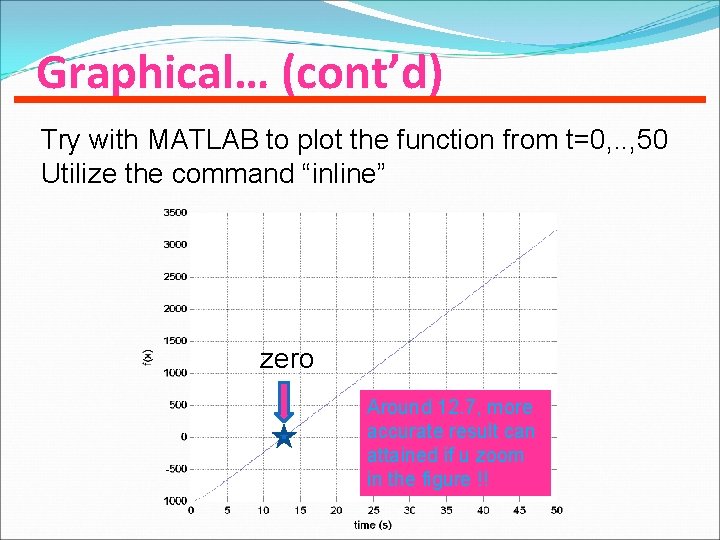
Graphical… (cont’d) Try with MATLAB to plot the function from t=0, . . , 50 Utilize the command “inline” zero Around 12. 7, more accurate result can attained if u zoom in the figure !!

Bisection

Bracketing… Sometimes called two-point method Underline principle Root of f (x) is bounded by {x. L, x. U} where f(x. L)f(x. U) < 0
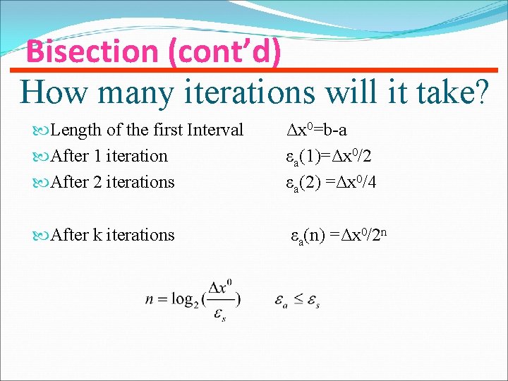
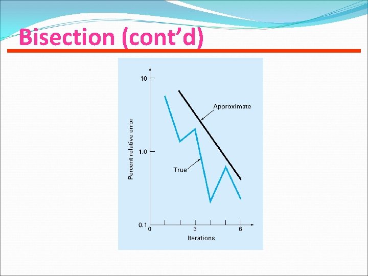
Bisection (cont’d) How many iterations will it take? Length of the first Interval After 1 iteration After 2 iterations Δx 0=b-a εa(1)=Δx 0/2 εa(2) =Δx 0/4 After k iterations εa(n) =Δx 0/2 n
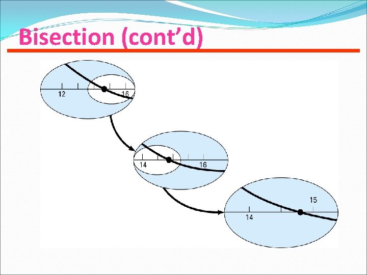
Bracketing: Bisection For the arbitrary equation of one variable, f(x)=0 1. Pick xl and xu such that they bound the root of interest, check if f(xl). f(xu) <0. 2. Estimate the root by evaluating f[(xl+xu)/2]. 3. Find the pair • If f(xl). f[(xl+xu)/2]<0, root lies in the lower interval, then xu=(xl+xu)/2 and go to step 2.
![Bisection (cont’d) • If f(xl). f[(xl+xu)/2]>0, root lies in the upper interval, then xl= Bisection (cont’d) • If f(xl). f[(xl+xu)/2]>0, root lies in the upper interval, then xl=](http://slidetodoc.com/presentation_image_h/d2464dab0c067ac207df6829319e9853/image-17.jpg)
Bisection (cont’d) • If f(xl). f[(xl+xu)/2]>0, root lies in the upper interval, then xl= [(xl+xu)/2, go to step 2. • If f(xl). f[(xl+xu)/2]=0, then root is (xl+xu)/2 and terminate. 4. Compare es with ea 5. If ea< es, stop. Otherwise repeat the process.
Bisection (cont’d)
Bisection (cont’d)
Bisection (cont’d) Evaluation of Method Pros Easy Always find root Number of iterations required to attain an absolute error can be computed a priori. Cons Slow Know a and b that bound root Multiple roots No account is taken of f(xl) and f(xu), if f(xl) is closer to zero, it is likely that root is closer to xl.
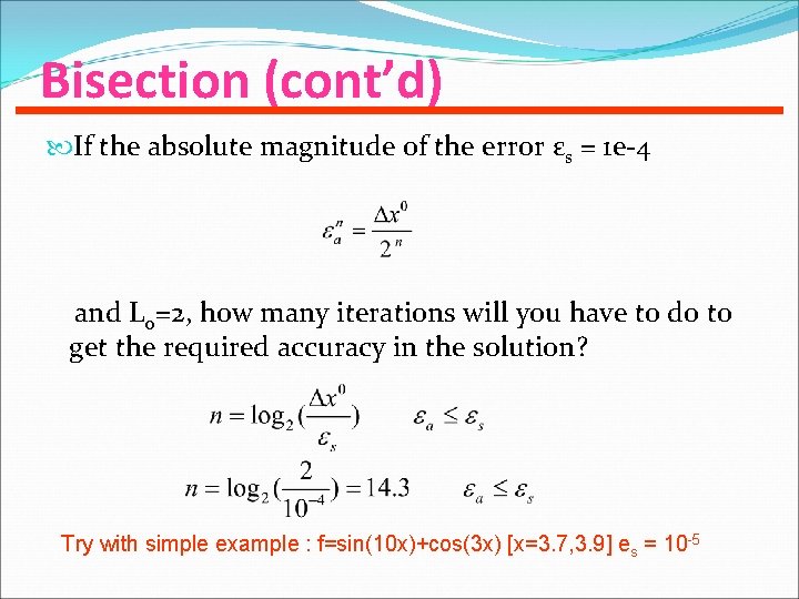
Bisection (cont’d) If the absolute magnitude of the error εs = 1 e-4 and Lo=2, how many iterations will you have to do to get the required accuracy in the solution? Try with simple example : f=sin(10 x)+cos(3 x) [x=3. 7, 3. 9] es = 10 -5
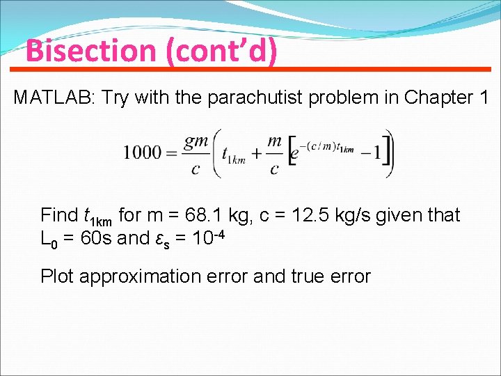
Bisection (cont’d) MATLAB: Try with the parachutist problem in Chapter 1 Find t 1 km for m = 68. 1 kg, c = 12. 5 kg/s given that L 0 = 60 s and εs = 10 -4 Plot approximation error and true error
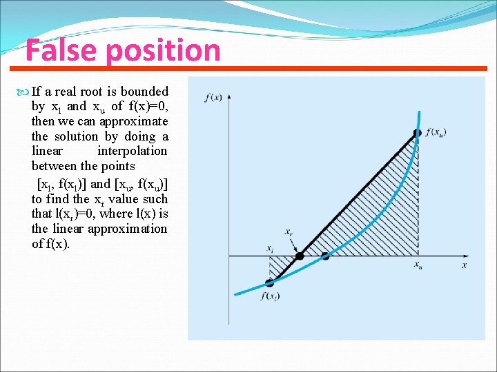
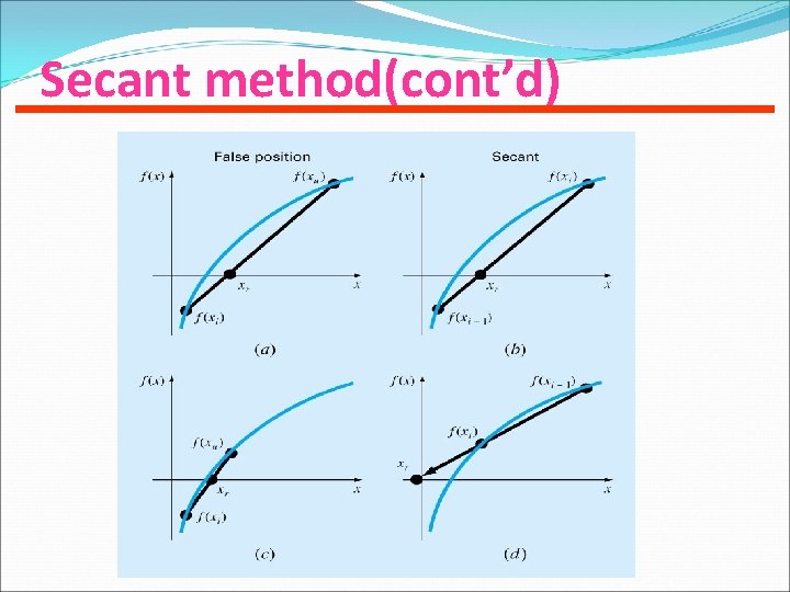
False position If a real root is bounded by xl and xu of f(x)=0, then we can approximate the solution by doing a linear interpolation between the points [xl, f(xl)] and [xu, f(xu)] to find the xr value such that l(xr)=0, where l(x) is the linear approximation of f(x).
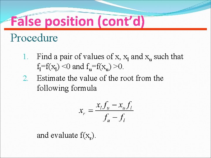
False position (cont’d) Procedure Find a pair of values of x, xl and xu such that fl=f(xl) <0 and fu=f(xu) >0. 2. Estimate the value of the root from the following formula 1. and evaluate f(xr).
False position (cont’d) Procedure (cont’d) 3. Use the new point to replace one of the original points, keeping the two points on opposite sides of the x axis. If f(xr)<0 then xl=xr == > fl=f(xr) If f(xr)>0 then xu=xr == > fu=f(xr) If f(xr)=0 then you have found the root and need go no further!
False position (cont’d) Procedure (cont’d) 4. See if the new xl and xu are close enough for convergence to be declared. If they are not go back to step 2. Now u may wonder how good of this technique is? Comparing with the bisection method, which one is better ? I would like u try this method with parachutist problem.
False position… (cont’d) Why this method? Faster Always converges for a single root. Pitfalls of the False-Position Method applied to some curvature functions may slowly converge.
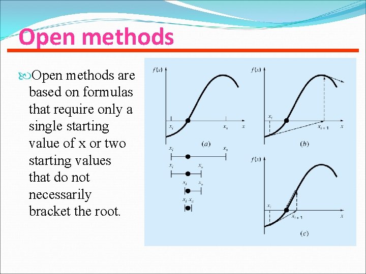
Open methods are based on formulas that require only a single starting value of x or two starting values that do not necessarily bracket the root.
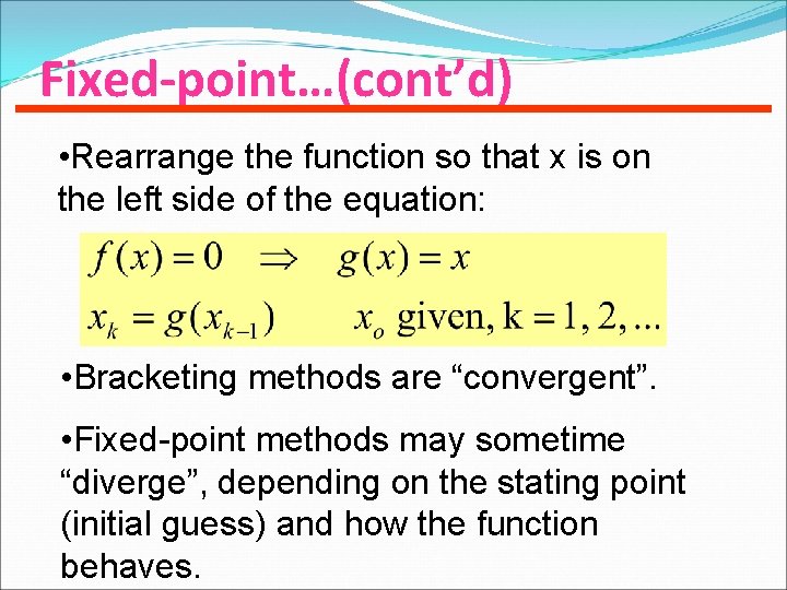
Fixed-point…(cont’d) • Rearrange the function so that x is on the left side of the equation: • Bracketing methods are “convergent”. • Fixed-point methods may sometime “diverge”, depending on the stating point (initial guess) and how the function behaves.
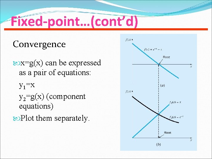
Fixed-point…(cont’d) Convergence x=g(x) can be expressed as a pair of equations: y 1=x y 2=g(x) (component equations) Plot them separately.
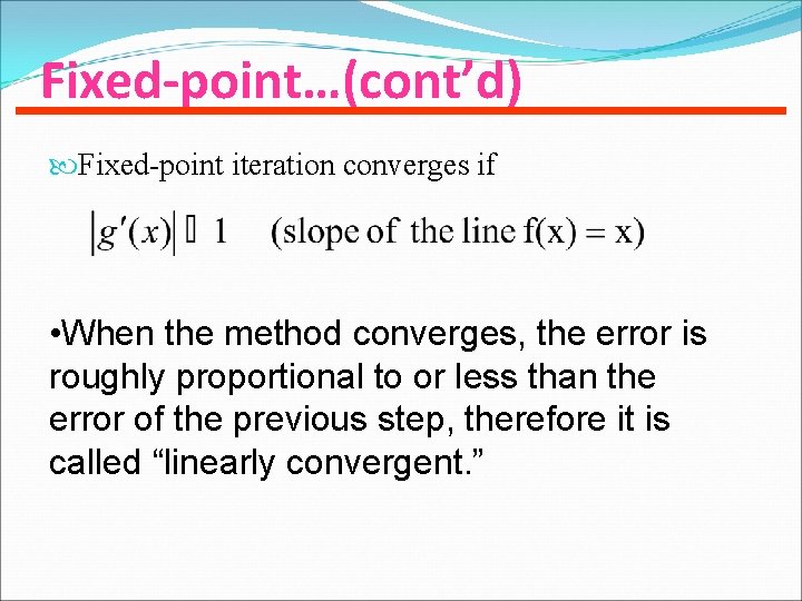
Fixed-point…(cont’d) Fixed-point iteration converges if • When the method converges, the error is roughly proportional to or less than the error of the previous step, therefore it is called “linearly convergent. ”
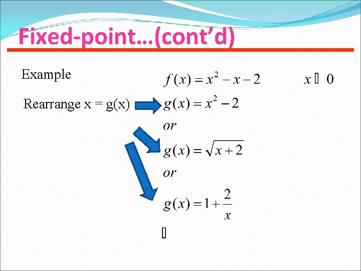
Fixed-point…(cont’d) Example Rearrange x = g(x)
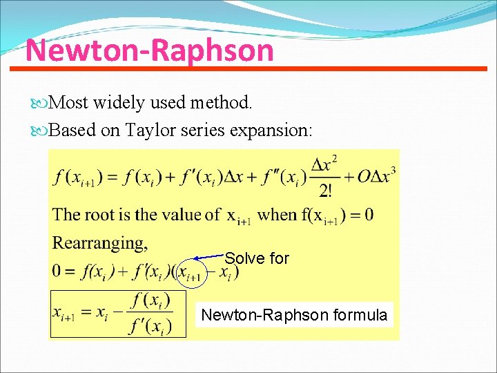
Newton-Raphson Most widely used method. Based on Taylor series expansion: Solve for Newton-Raphson formula
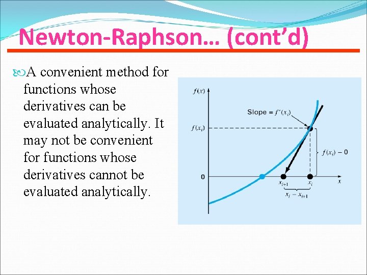
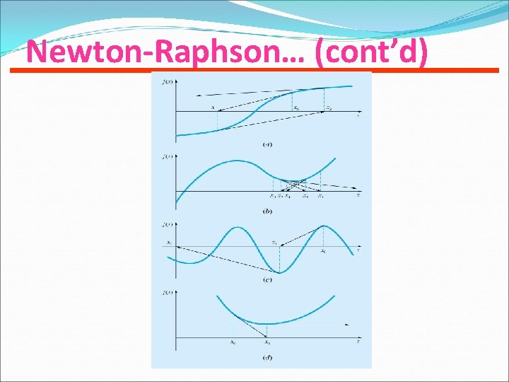
Newton-Raphson… (cont’d) A convenient method for functions whose derivatives can be evaluated analytically. It may not be convenient for functions whose derivatives cannot be evaluated analytically.
Newton-Raphson… (cont’d)
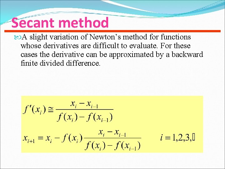
Secant method A slight variation of Newton’s method for functions whose derivatives are difficult to evaluate. For these cases the derivative can be approximated by a backward finite divided difference.

Secant method(cont’d) • Requires two initial estimates of x , e. g, xo, x 1. However, because f(x) is not required to change signs between estimates, it is not classified as a “bracketing” method. • The scant method has the same properties as Newton’s method. Convergence is not guaranteed for all xo, f(x).
Secant method(cont’d)
- Slides: 38