Chapter 3 Rational Consumer Choice Chapter Outline The

Chapter 3 Rational Consumer Choice

Chapter Outline • • • The Opportunity Set or Budget Constraint Budget Shifts Due to Price or Income Changes Consumer Preferences The Best Feasible Bundle Appendix: – The Utility Function Approach to the Consumer Choice – Cardinal versus Ordinal Utility – Generating Indifference Curves Algebraically © 2015 Mc. Graw-Hill Education. All Rights Reserved. 2

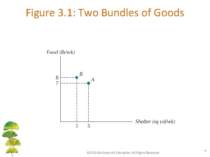
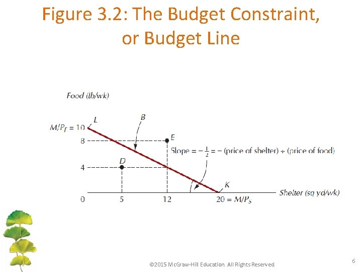
Budget Limitation • A bundle: a particular combination of two or more goods. • Budget constraint: the set of all bundles that exactly exhaust the consumer’s income at given prices. – Its slope is the negative of the price ratio of the two goods. © 2015 Mc. Graw-Hill Education. All Rights Reserved. 3

Figure 3. 1: Two Bundles of Goods © 2015 Mc. Graw-Hill Education. All Rights Reserved. 4

Affordable vs. Unaffordable • Affordable set, or feasible set: bundles on or below the budget constraint; bundles for which the required expenditure at given prices is less than or equal to the income available. • Unaffordable set, or unfeasible set: bundles that lie outside the budget constraint © 2015 Mc. Graw-Hill Education. All Rights Reserved. 5

Figure 3. 2: The Budget Constraint, or Budget Line © 2015 Mc. Graw-Hill Education. All Rights Reserved. 6

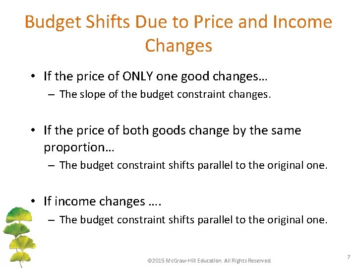
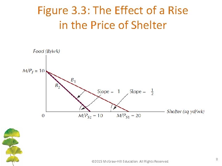
Budget Shifts Due to Price and Income Changes • If the price of ONLY one good changes… – The slope of the budget constraint changes. • If the price of both goods change by the same proportion… – The budget constraint shifts parallel to the original one. • If income changes …. – The budget constraint shifts parallel to the original one. © 2015 Mc. Graw-Hill Education. All Rights Reserved. 7

Figure 3. 3: The Effect of a Rise in the Price of Shelter © 2015 Mc. Graw-Hill Education. All Rights Reserved. 8

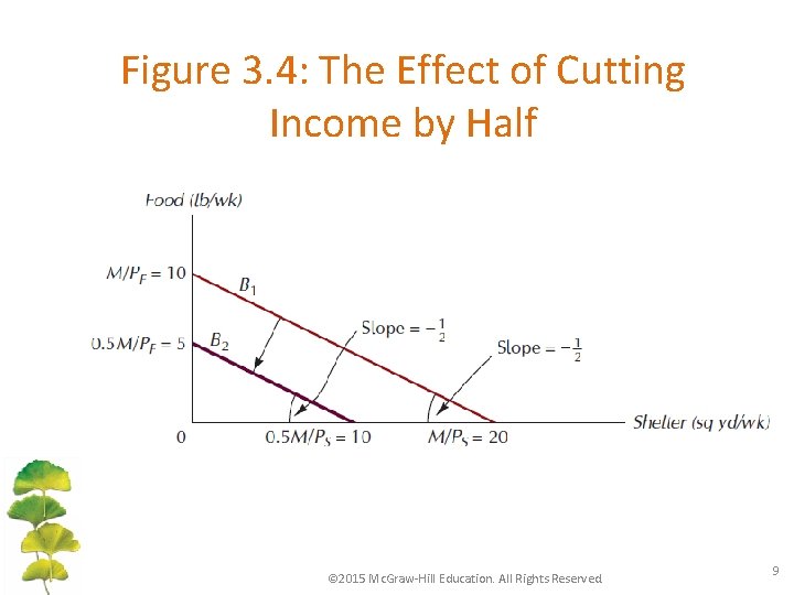
Figure 3. 4: The Effect of Cutting Income by Half © 2015 Mc. Graw-Hill Education. All Rights Reserved. 9

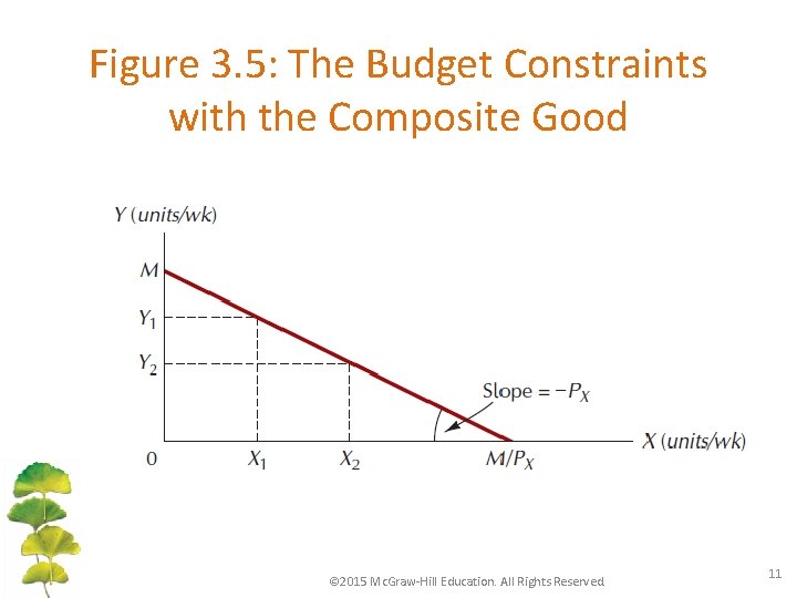
Budgets Involving More Than Two Goods • When we have more than 3 goods, the budget constraint becomes a hyperplane, or multidimensional plane. • In this case, view the consumer’s choice as one between a good, X, and an amalgam of other goods, Y. This amalgam is called the composite good. – The amount of income left after buying good X – The amount the consumer spends on goods other than good X © 2015 Mc. Graw-Hill Education. All Rights Reserved. 10

Figure 3. 5: The Budget Constraints with the Composite Good © 2015 Mc. Graw-Hill Education. All Rights Reserved. 11

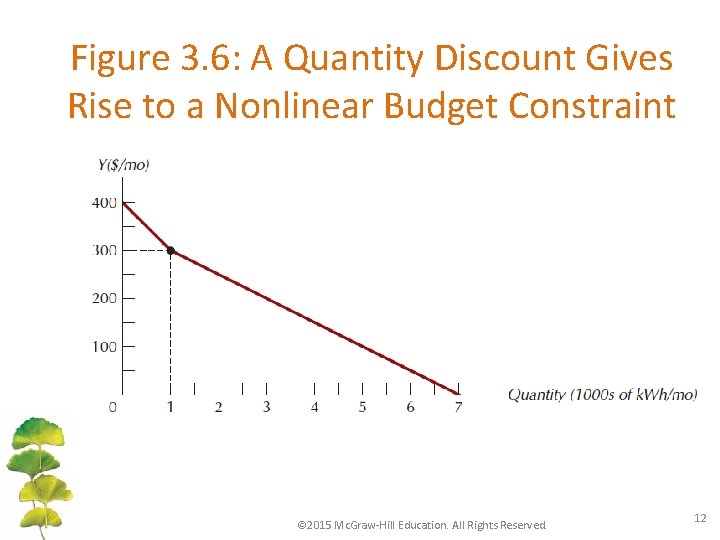
Figure 3. 6: A Quantity Discount Gives Rise to a Nonlinear Budget Constraint © 2015 Mc. Graw-Hill Education. All Rights Reserved. 12

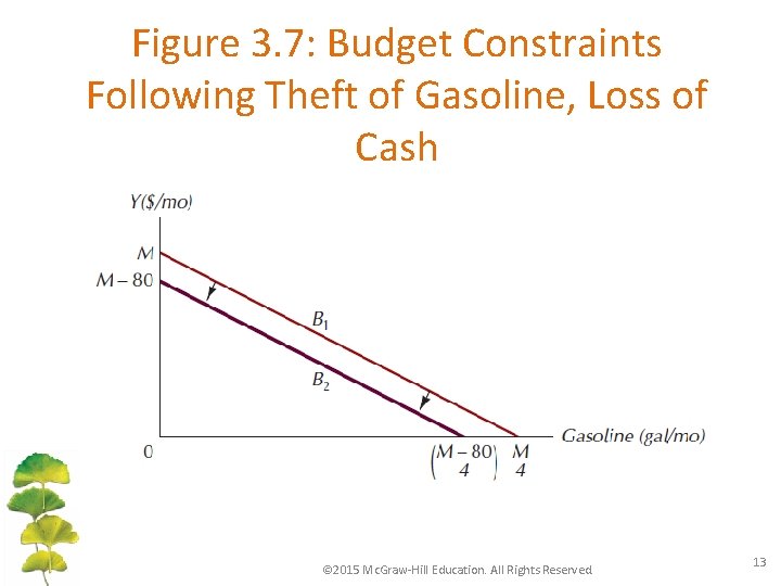
Figure 3. 7: Budget Constraints Following Theft of Gasoline, Loss of Cash © 2015 Mc. Graw-Hill Education. All Rights Reserved. 13

Preference Ordering • Preference ordering: a ranking of all possible consumption bundles in order of preference. – Differ widely among consumers – Four simple properties of preference ordering © 2015 Mc. Graw-Hill Education. All Rights Reserved. 14

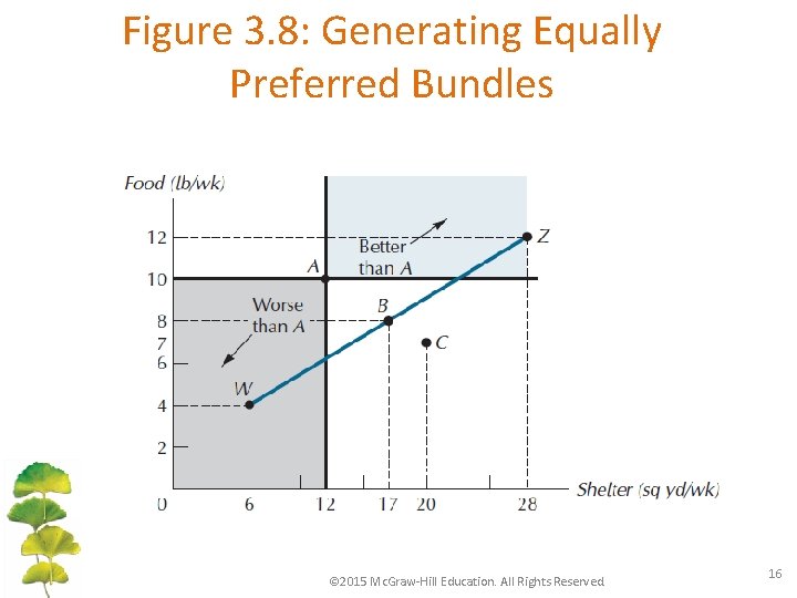
Properties of Preference Orderings • Completeness: the consumer is able to rank all possible combinations of goods and services. • More-Is-Better: other things equal, more of a good is preferred to less. • Transitivity: for any three bundles A, B, and C, if he prefers A to B and prefers B to C, then he always prefers A to C. • Convexity: mixtures of goods are preferable to extremes. © 2015 Mc. Graw-Hill Education. All Rights Reserved. 15

Figure 3. 8: Generating Equally Preferred Bundles © 2015 Mc. Graw-Hill Education. All Rights Reserved. 16

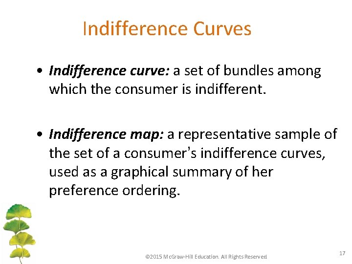
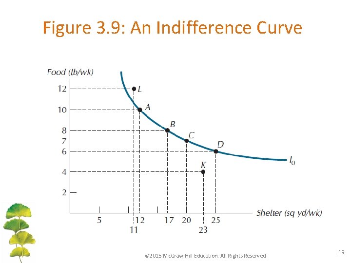
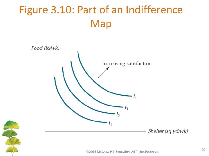
Indifference Curves • Indifference curve: a set of bundles among which the consumer is indifferent. • Indifference map: a representative sample of the set of a consumer’s indifference curves, used as a graphical summary of her preference ordering. © 2015 Mc. Graw-Hill Education. All Rights Reserved. 17

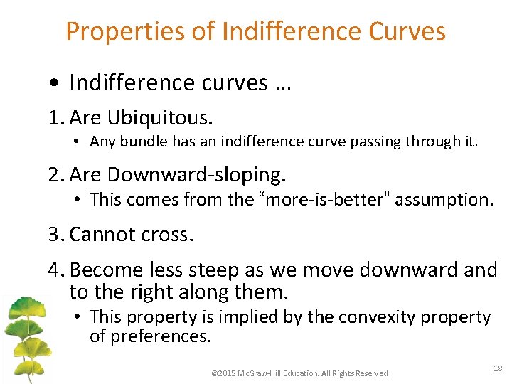
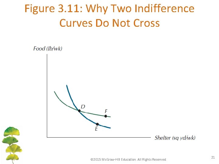
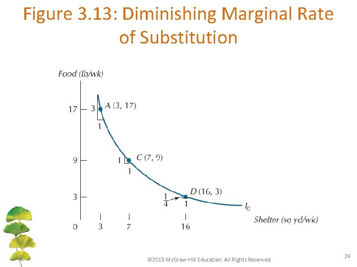
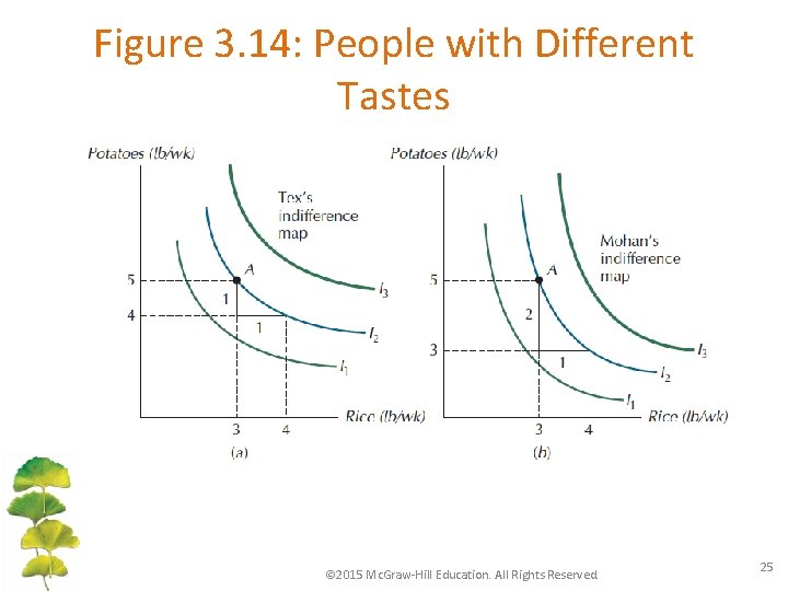
Properties of Indifference Curves • Indifference curves … 1. Are Ubiquitous. • Any bundle has an indifference curve passing through it. 2. Are Downward-sloping. • This comes from the “more-is-better” assumption. 3. Cannot cross. 4. Become less steep as we move downward and to the right along them. • This property is implied by the convexity property of preferences. © 2015 Mc. Graw-Hill Education. All Rights Reserved. 18

Figure 3. 9: An Indifference Curve © 2015 Mc. Graw-Hill Education. All Rights Reserved. 19

Figure 3. 10: Part of an Indifference Map © 2015 Mc. Graw-Hill Education. All Rights Reserved. 20

Figure 3. 11: Why Two Indifference Curves Do Not Cross © 2015 Mc. Graw-Hill Education. All Rights Reserved. 21

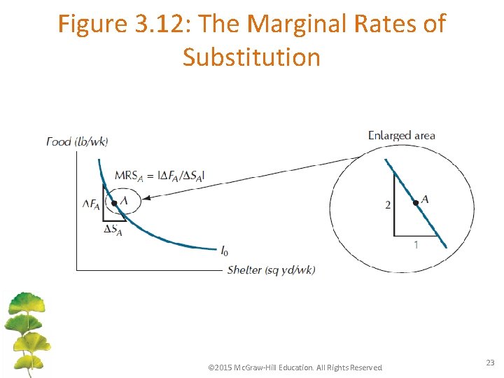
Trade-offs Between Goods • Marginal rate of substitution (MRS): the rate at which the consumer is willing to exchange the good measured along the vertical axis for the good measured along the horizontal axis. – Equal to the absolute value of the slope of the indifference curve. © 2015 Mc. Graw-Hill Education. All Rights Reserved. 22

Figure 3. 12: The Marginal Rates of Substitution © 2015 Mc. Graw-Hill Education. All Rights Reserved. 23

Figure 3. 13: Diminishing Marginal Rate of Substitution © 2015 Mc. Graw-Hill Education. All Rights Reserved. 24

Figure 3. 14: People with Different Tastes © 2015 Mc. Graw-Hill Education. All Rights Reserved. 25

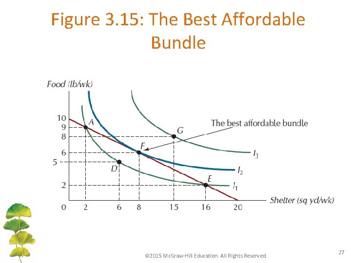
The Best Feasible Bundle • Consumer’s Goal: to choose the best affordable bundle. – The same as reaching the highest indifference curve she can, given her budget constraint. – For convex indifference curves. . • the best bundle will always lie at the point of tangency. © 2015 Mc. Graw-Hill Education. All Rights Reserved. 26

Figure 3. 15: The Best Affordable Bundle © 2015 Mc. Graw-Hill Education. All Rights Reserved. 27

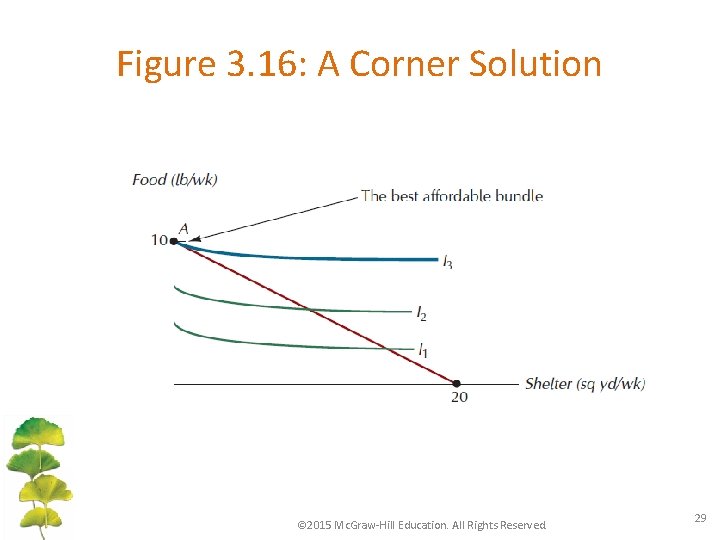
Corner Solutions • Corner solution: in a choice between two goods, a case in which the consumer does not consume one of the goods. © 2015 Mc. Graw-Hill Education. All Rights Reserved. 28

Figure 3. 16: A Corner Solution © 2015 Mc. Graw-Hill Education. All Rights Reserved. 29

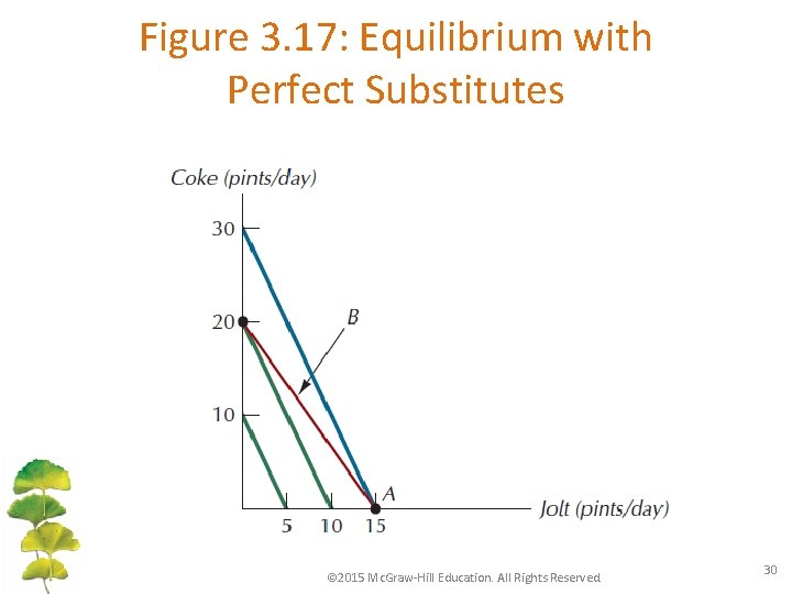
Figure 3. 17: Equilibrium with Perfect Substitutes © 2015 Mc. Graw-Hill Education. All Rights Reserved. 30

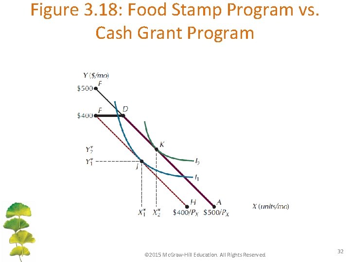
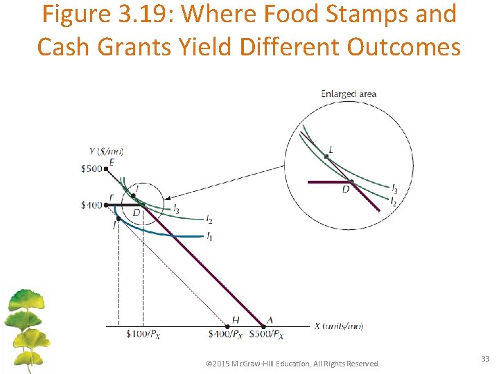
Cash or Food Stamps? • Food Stamp Program – Objective - to alleviate hunger. – How does it work? • People whose incomes fall below a certain level are eligible to receive a specified quantity of food stamps. • Stamps cannot be used to purchase cigarettes, alcohol, and various other items. • The government gives food retailers cash for the stamps they accept. © 2015 Mc. Graw-Hill Education. All Rights Reserved. 31

Figure 3. 18: Food Stamp Program vs. Cash Grant Program © 2015 Mc. Graw-Hill Education. All Rights Reserved. 32

Figure 3. 19: Where Food Stamps and Cash Grants Yield Different Outcomes © 2015 Mc. Graw-Hill Education. All Rights Reserved. 33

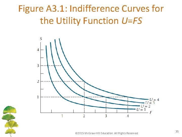
The Utility Function Approach to Consumer Choice • Finding the highest attainable indifference curve on a budget constraint is just one way to analyze the consumer choice problem • In this second approach, we represent the consumer’s preference not with an indifference map, but with a utility function. © 2015 Mc. Graw-Hill Education. All Rights Reserved. 34

Figure A 3. 1: Indifference Curves for the Utility Function U=FS © 2015 Mc. Graw-Hill Education. All Rights Reserved. 35

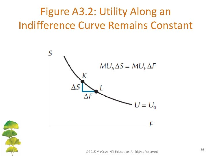
Figure A 3. 2: Utility Along an Indifference Curve Remains Constant © 2015 Mc. Graw-Hill Education. All Rights Reserved. 36

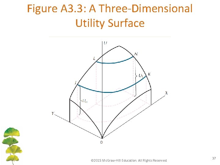
Figure A 3. 3: A Three-Dimensional Utility Surface © 2015 Mc. Graw-Hill Education. All Rights Reserved. 37

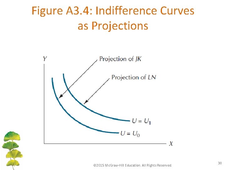
Figure A 3. 4: Indifference Curves as Projections © 2015 Mc. Graw-Hill Education. All Rights Reserved. 38

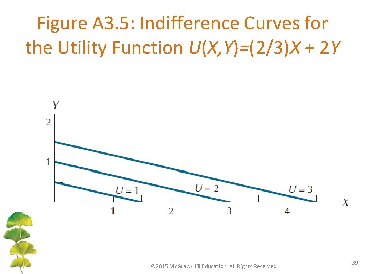
Figure A 3. 5: Indifference Curves for the Utility Function U(X, Y)=(2/3)X + 2 Y © 2015 Mc. Graw-Hill Education. All Rights Reserved. 39

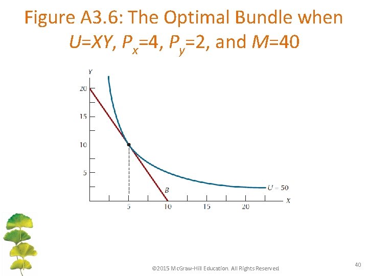
Figure A 3. 6: The Optimal Bundle when U=XY, Px=4, Py=2, and M=40 © 2015 Mc. Graw-Hill Education. All Rights Reserved. 40