Chapter 3 Quadratic Functions and Equations Copyright 2014
- Slides: 38

Chapter 3 Quadratic Functions and Equations Copyright © 2014, 2010, 2006 Pearson Education, Inc. 1

3. 5 ♦ ♦ ♦ Transformations of Graphs Graph functions using vertical and horizontal shifts Graph functions using stretching and shrinking Graph functions using reflections Combine transformations Model data with transformations (optional) Copyright © 2014, 2010, 2006 Pearson Education, Inc. 2

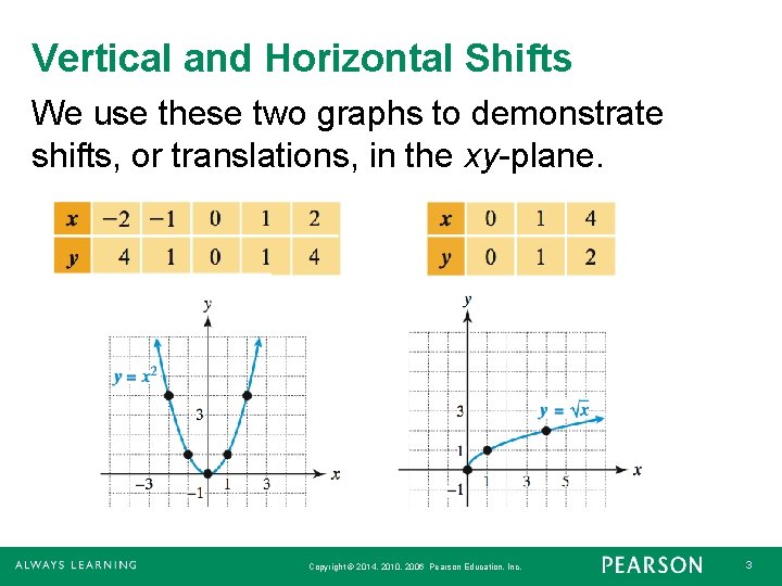
Vertical and Horizontal Shifts We use these two graphs to demonstrate shifts, or translations, in the xy-plane. Copyright © 2014, 2010, 2006 Pearson Education, Inc. 3

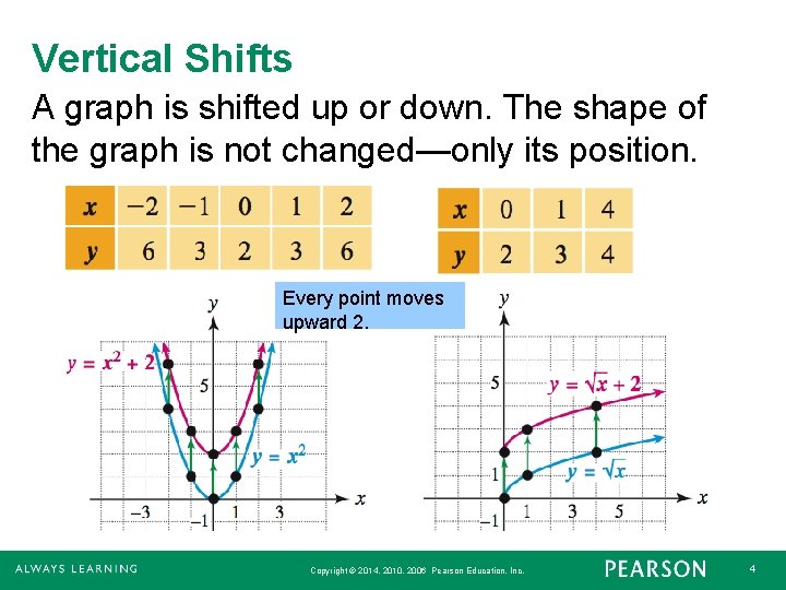
Vertical Shifts A graph is shifted up or down. The shape of the graph is not changed—only its position. Every point moves upward 2. Copyright © 2014, 2010, 2006 Pearson Education, Inc. 4

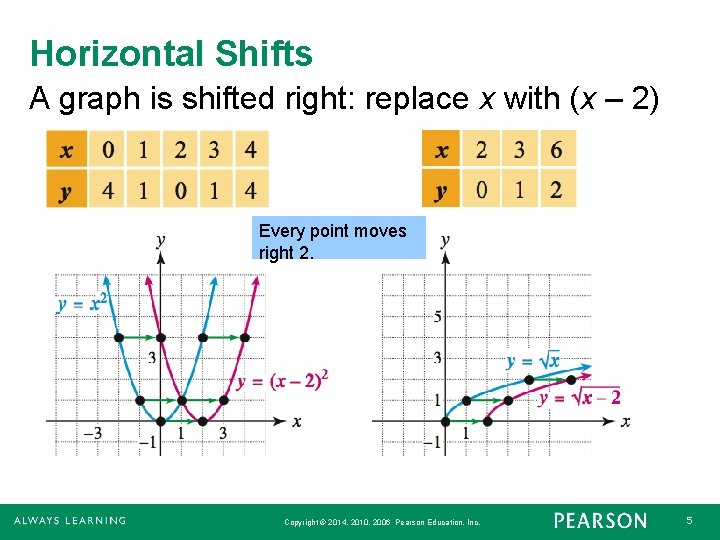
Horizontal Shifts A graph is shifted right: replace x with (x – 2) Every point moves right 2. Copyright © 2014, 2010, 2006 Pearson Education, Inc. 5

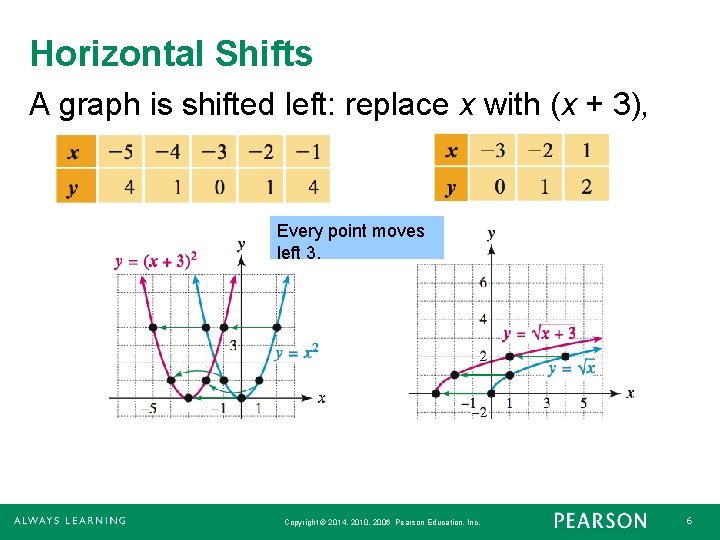
Horizontal Shifts A graph is shifted left: replace x with (x + 3), Every point moves left 3. Copyright © 2014, 2010, 2006 Pearson Education, Inc. 6

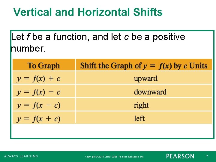
Vertical and Horizontal Shifts Let f be a function, and let c be a positive number. Copyright © 2014, 2010, 2006 Pearson Education, Inc. 7

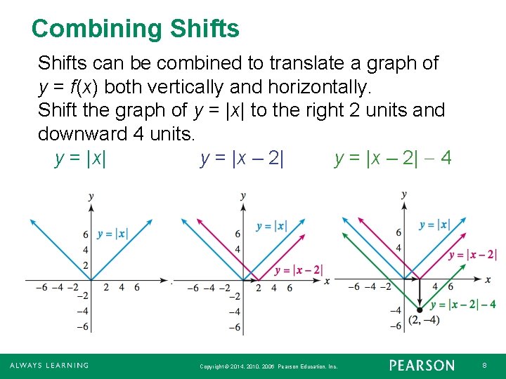
Combining Shifts can be combined to translate a graph of y = f(x) both vertically and horizontally. Shift the graph of y = |x| to the right 2 units and downward 4 units. y = |x| y = |x – 2| 4 Copyright © 2014, 2010, 2006 Pearson Education, Inc. 8

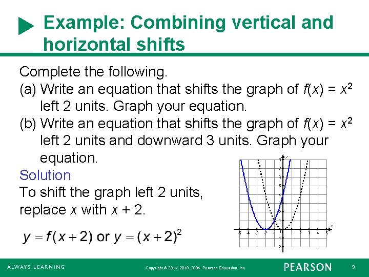
Example: Combining vertical and horizontal shifts Complete the following. (a) Write an equation that shifts the graph of f(x) = x 2 left 2 units. Graph your equation. (b) Write an equation that shifts the graph of f(x) = x 2 left 2 units and downward 3 units. Graph your equation. Solution To shift the graph left 2 units, replace x with x + 2. Copyright © 2014, 2010, 2006 Pearson Education, Inc. 9

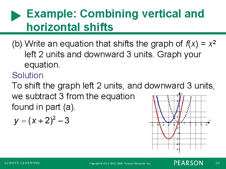
Example: Combining vertical and horizontal shifts (b) Write an equation that shifts the graph of f(x) = x 2 left 2 units and downward 3 units. Graph your equation. Solution To shift the graph left 2 units, and downward 3 units, we subtract 3 from the equation found in part (a). Copyright © 2014, 2010, 2006 Pearson Education, Inc. 10

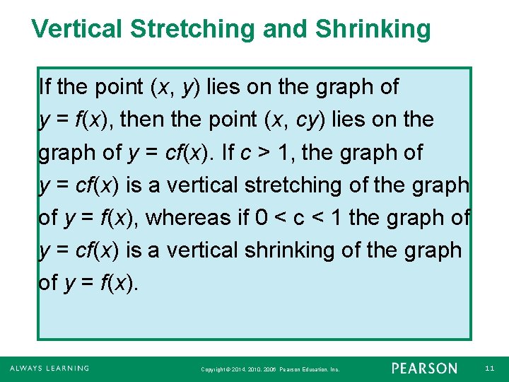
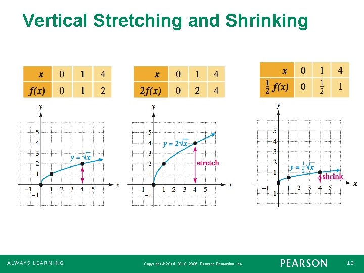
Vertical Stretching and Shrinking If the point (x, y) lies on the graph of y = f(x), then the point (x, cy) lies on the graph of y = cf(x). If c > 1, the graph of y = cf(x) is a vertical stretching of the graph of y = f(x), whereas if 0 < c < 1 the graph of y = cf(x) is a vertical shrinking of the graph of y = f(x). Copyright © 2014, 2010, 2006 Pearson Education, Inc. 11

Vertical Stretching and Shrinking Copyright © 2014, 2010, 2006 Pearson Education, Inc. 12

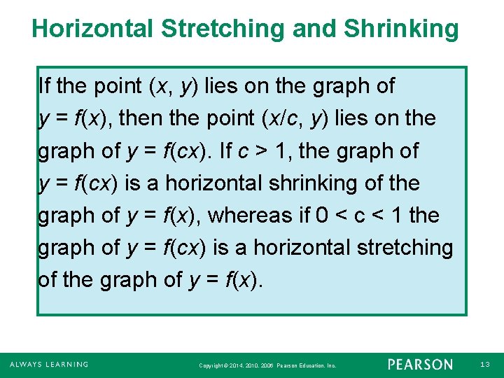
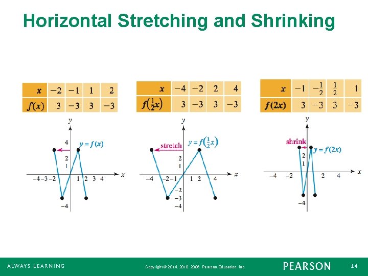
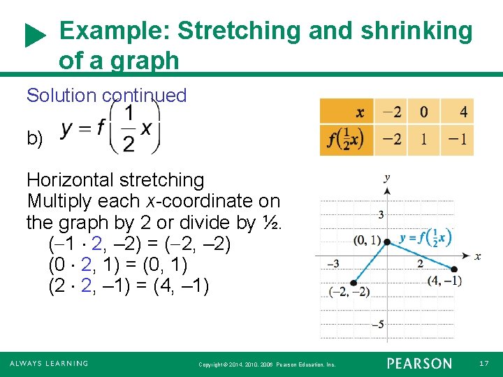
Horizontal Stretching and Shrinking If the point (x, y) lies on the graph of y = f(x), then the point (x/c, y) lies on the graph of y = f(cx). If c > 1, the graph of y = f(cx) is a horizontal shrinking of the graph of y = f(x), whereas if 0 < c < 1 the graph of y = f(cx) is a horizontal stretching of the graph of y = f(x). Copyright © 2014, 2010, 2006 Pearson Education, Inc. 13

Horizontal Stretching and Shrinking Copyright © 2014, 2010, 2006 Pearson Education, Inc. 14

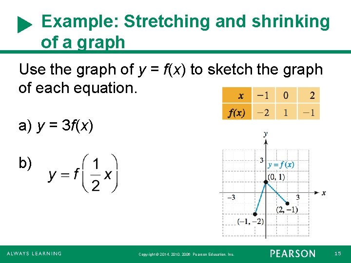
Example: Stretching and shrinking of a graph Use the graph of y = f(x) to sketch the graph of each equation. a) y = 3 f(x) b) Copyright © 2014, 2010, 2006 Pearson Education, Inc. 15

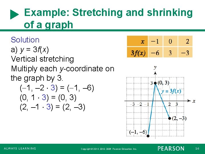
Example: Stretching and shrinking of a graph Solution a) y = 3 f(x) Vertical stretching Multiply each y-coordinate on the graph by 3. ( 1, – 2 3) = ( 1, – 6) (0, 1 3) = (0, 3) (2, – 1 3) = (2, – 3) Copyright © 2014, 2010, 2006 Pearson Education, Inc. 16

Example: Stretching and shrinking of a graph Solution continued b) Horizontal stretching Multiply each x-coordinate on the graph by 2 or divide by ½. ( 1 2, – 2) = ( 2, – 2) (0 2, 1) = (0, 1) (2 2, – 1) = (4, – 1) Copyright © 2014, 2010, 2006 Pearson Education, Inc. 17

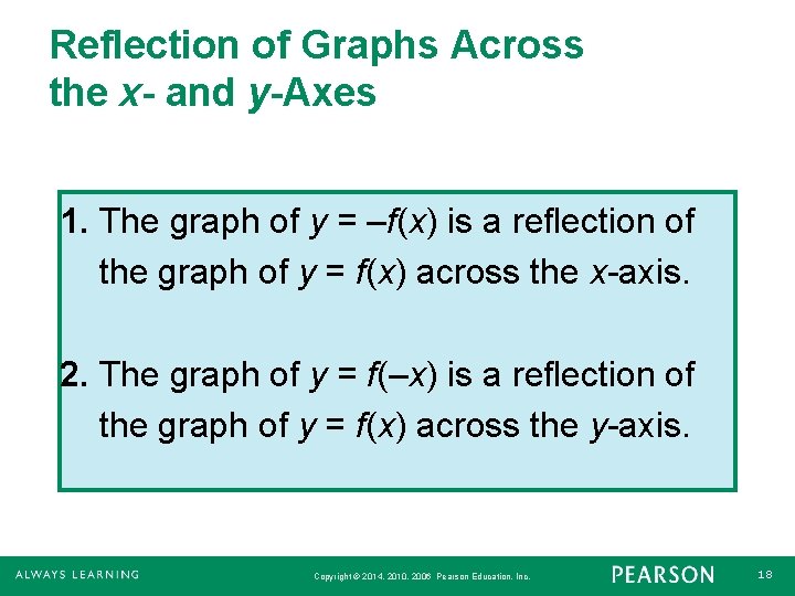
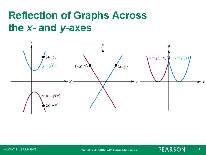
Reflection of Graphs Across the x- and y-Axes 1. The graph of y = –f(x) is a reflection of the graph of y = f(x) across the x-axis. 2. The graph of y = f(–x) is a reflection of the graph of y = f(x) across the y-axis. Copyright © 2014, 2010, 2006 Pearson Education, Inc. 18

Reflection of Graphs Across the x- and y-axes Copyright © 2014, 2010, 2006 Pearson Education, Inc. 19

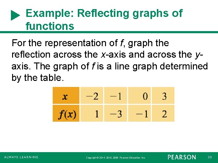
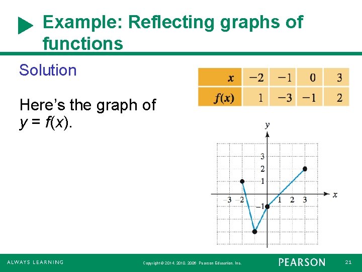
Example: Reflecting graphs of functions For the representation of f, graph the reflection across the x-axis and across the yaxis. The graph of f is a line graph determined by the table. Copyright © 2014, 2010, 2006 Pearson Education, Inc. 20

Example: Reflecting graphs of functions Solution Here’s the graph of y = f(x). Copyright © 2014, 2010, 2006 Pearson Education, Inc. 21

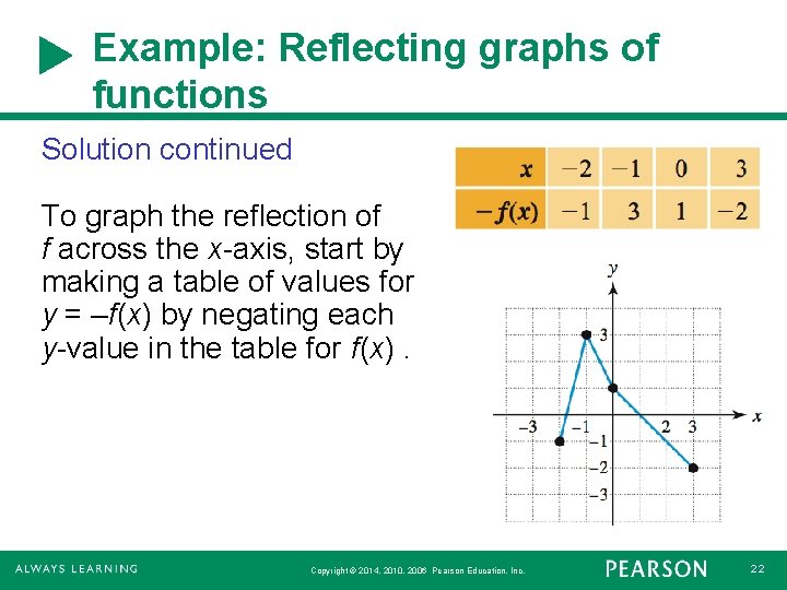
Example: Reflecting graphs of functions Solution continued To graph the reflection of f across the x-axis, start by making a table of values for y = –f(x) by negating each y-value in the table for f(x). Copyright © 2014, 2010, 2006 Pearson Education, Inc. 22

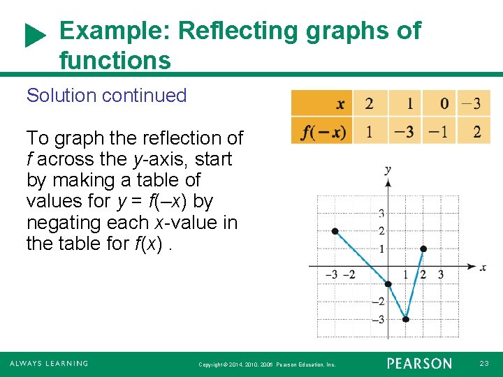
Example: Reflecting graphs of functions Solution continued To graph the reflection of f across the y-axis, start by making a table of values for y = f(–x) by negating each x-value in the table for f(x). Copyright © 2014, 2010, 2006 Pearson Education, Inc. 23

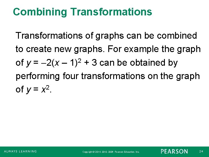
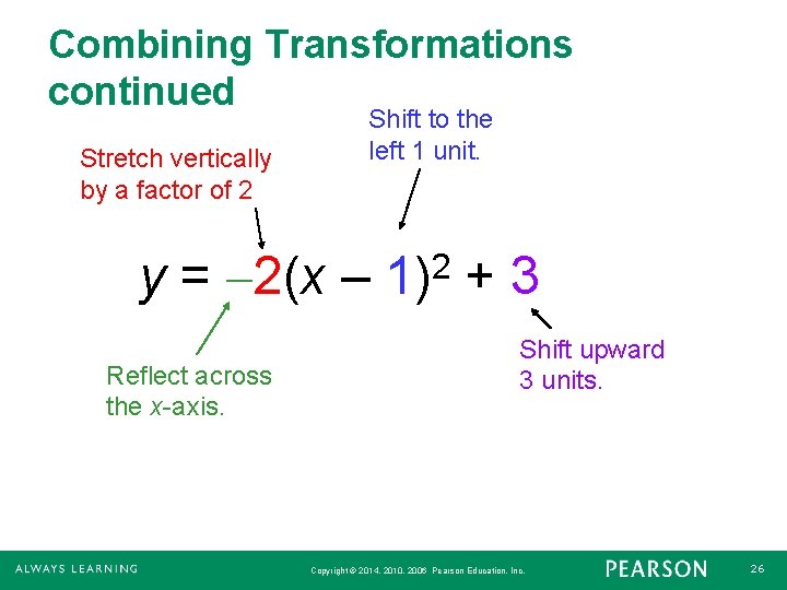
Combining Transformations of graphs can be combined to create new graphs. For example the graph of y = 2(x – 1)2 + 3 can be obtained by performing four transformations on the graph of y = x 2. Copyright © 2014, 2010, 2006 Pearson Education, Inc. 24

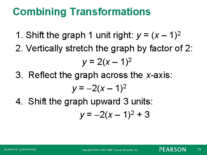
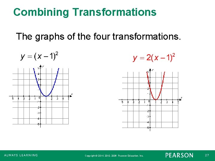
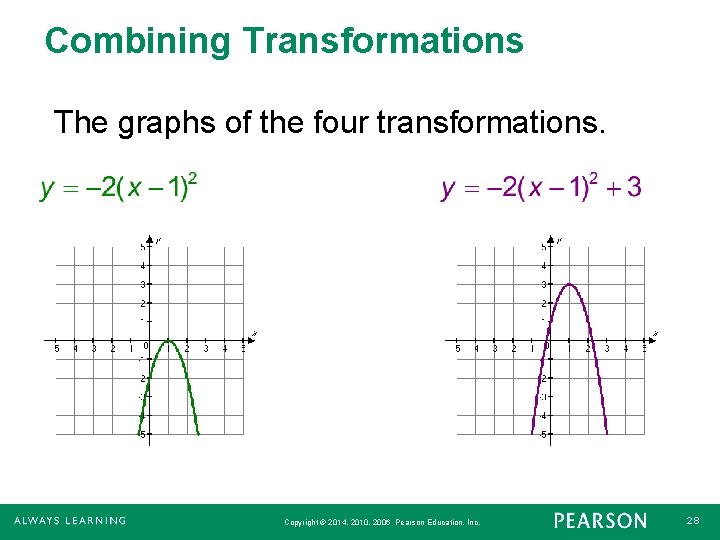
Combining Transformations 1. Shift the graph 1 unit right: y = (x – 1)2 2. Vertically stretch the graph by factor of 2: y = 2(x – 1)2 3. Reflect the graph across the x-axis: y = 2(x – 1)2 4. Shift the graph upward 3 units: y = 2(x – 1)2 + 3 Copyright © 2014, 2010, 2006 Pearson Education, Inc. 25

Combining Transformations continued Stretch vertically by a factor of 2 Shift to the left 1 unit. y = 2(x – Reflect across the x-axis. 2 1) +3 Shift upward 3 units. Copyright © 2014, 2010, 2006 Pearson Education, Inc. 26

Combining Transformations The graphs of the four transformations. Copyright © 2014, 2010, 2006 Pearson Education, Inc. 27

Combining Transformations The graphs of the four transformations. Copyright © 2014, 2010, 2006 Pearson Education, Inc. 28

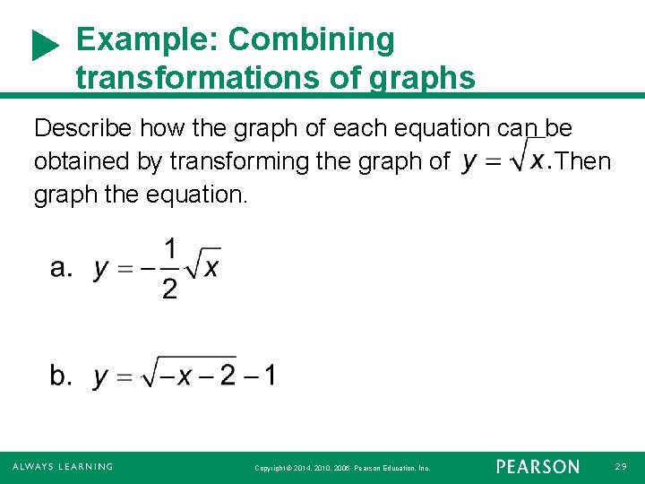
Example: Combining transformations of graphs Describe how the graph of each equation can be obtained by transforming the graph of Then graph the equation. Copyright © 2014, 2010, 2006 Pearson Education, Inc. 29

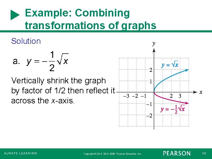
Example: Combining transformations of graphs Solution Vertically shrink the graph by factor of 1/2 then reflect it across the x-axis. Copyright © 2014, 2010, 2006 Pearson Education, Inc. 30

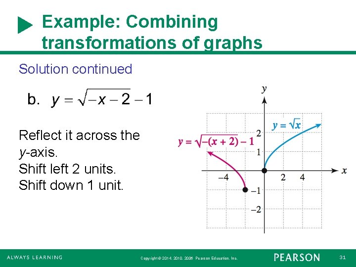
Example: Combining transformations of graphs Solution continued Reflect it across the y-axis. Shift left 2 units. Shift down 1 unit. Copyright © 2014, 2010, 2006 Pearson Education, Inc. 31

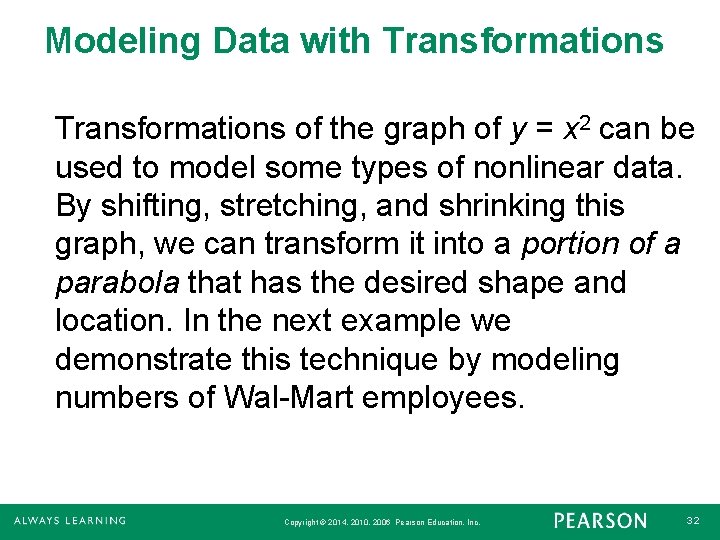
Modeling Data with Transformations of the graph of y = x 2 can be used to model some types of nonlinear data. By shifting, stretching, and shrinking this graph, we can transform it into a portion of a parabola that has the desired shape and location. In the next example we demonstrate this technique by modeling numbers of Wal-Mart employees. Copyright © 2014, 2010, 2006 Pearson Education, Inc. 32

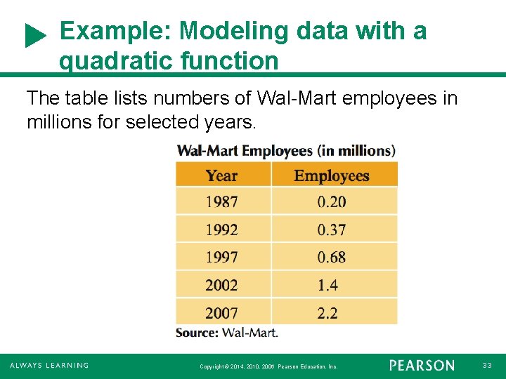
Example: Modeling data with a quadratic function The table lists numbers of Wal-Mart employees in millions for selected years. Copyright © 2014, 2010, 2006 Pearson Education, Inc. 33

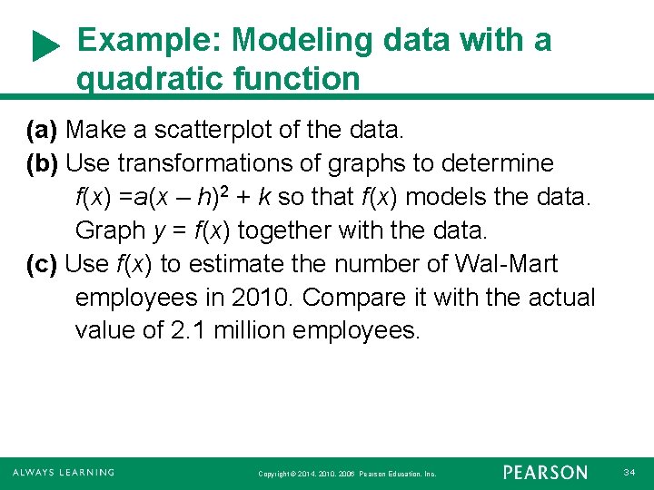
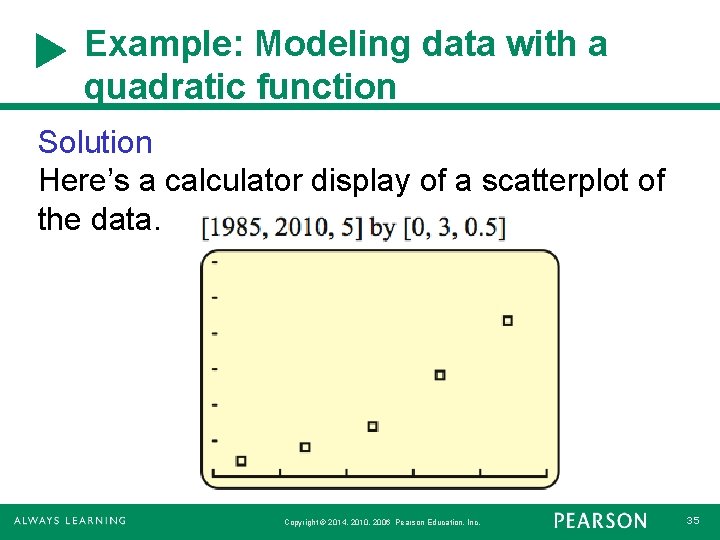
Example: Modeling data with a quadratic function (a) Make a scatterplot of the data. (b) Use transformations of graphs to determine f(x) =a(x – h)2 + k so that f(x) models the data. Graph y = f(x) together with the data. (c) Use f(x) to estimate the number of Wal-Mart employees in 2010. Compare it with the actual value of 2. 1 million employees. Copyright © 2014, 2010, 2006 Pearson Education, Inc. 34

Example: Modeling data with a quadratic function Solution Here’s a calculator display of a scatterplot of the data. Copyright © 2014, 2010, 2006 Pearson Education, Inc. 35

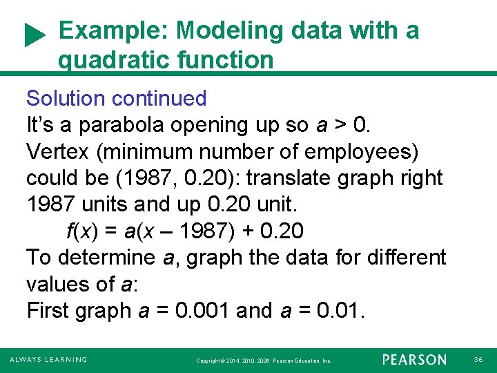
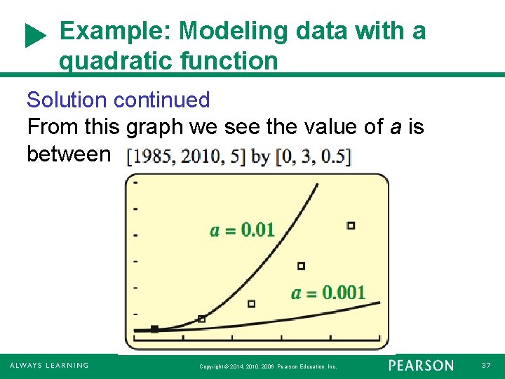
Example: Modeling data with a quadratic function Solution continued It’s a parabola opening up so a > 0. Vertex (minimum number of employees) could be (1987, 0. 20): translate graph right 1987 units and up 0. 20 unit. f(x) = a(x – 1987) + 0. 20 To determine a, graph the data for different values of a: First graph a = 0. 001 and a = 0. 01. Copyright © 2014, 2010, 2006 Pearson Education, Inc. 36

Example: Modeling data with a quadratic function Solution continued From this graph we see the value of a is between 0. 001 and 0. 01. Copyright © 2014, 2010, 2006 Pearson Education, Inc. 37

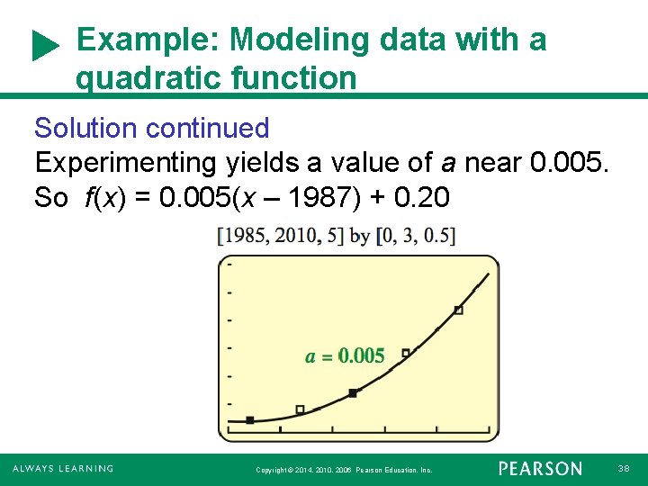
Example: Modeling data with a quadratic function Solution continued Experimenting yields a value of a near 0. 005. So f(x) = 0. 005(x – 1987) + 0. 20 Copyright © 2014, 2010, 2006 Pearson Education, Inc. 38