Chapter 3 PREFERENCES AND UTILITY Copyright 2005 by

Axioms of Rational Choice • Completeness – if A and B are any two situations, an individual can always specify exactly one of these possibilities: • A is preferred to B • B is preferred to A • A and B are equally attractive 2

Axioms of Rational Choice • Transitivity – if A is preferred to B, and B is preferred to C, then A is preferred to C – assumes that the individual’s choices are internally consistent 3

Axioms of Rational Choice • Continuity – if A is preferred to B, then situations suitably “close to” A must also be preferred to B – used to analyze individuals’ responses to relatively small changes in income and prices 4

Utility • Given these assumptions, it is possible to show that people are able to rank in order all possible situations from least desirable to most • Economists call this ranking utility – if A is preferred to B, then the utility assigned to A exceeds the utility assigned to B U(A) > U(B) 5

Utility • Utility rankings are ordinal in nature – they record the relative desirability of commodity bundles • Because utility measures are not unique, it makes no sense to consider how much more utility is gained from A than from B • It is also impossible to compare utilities between people 6

Utility • Utility is affected by the consumption of physical commodities, psychological attitudes, peer group pressures, personal experiences, and the general cultural environment • Economists generally devote attention to quantifiable options while holding constant the other things that affect utility – ceteris paribus assumption 7

Utility • Assume that an individual must choose among consumption goods x 1, x 2, …, xn • The individual’s rankings can be shown by a utility function of the form: utility = U(x 1, x 2, …, xn; other things) – this function is unique up to an orderpreserving transformation 8

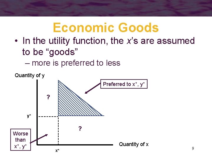
Economic Goods • In the utility function, the x’s are assumed to be “goods” – more is preferred to less Quantity of y Preferred to x*, y* ? y* Worse than x*, y* ? Quantity of x x* 9

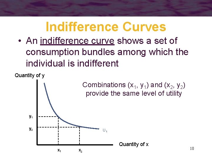
Indifference Curves • An indifference curve shows a set of consumption bundles among which the individual is indifferent Quantity of y Combinations (x 1, y 1) and (x 2, y 2) provide the same level of utility y 1 y 2 U 1 Quantity of x x 1 x 2 10

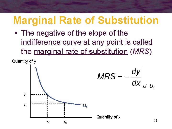
Marginal Rate of Substitution • The negative of the slope of the indifference curve at any point is called the marginal rate of substitution (MRS) Quantity of y y 1 y 2 U 1 Quantity of x x 1 x 2 11

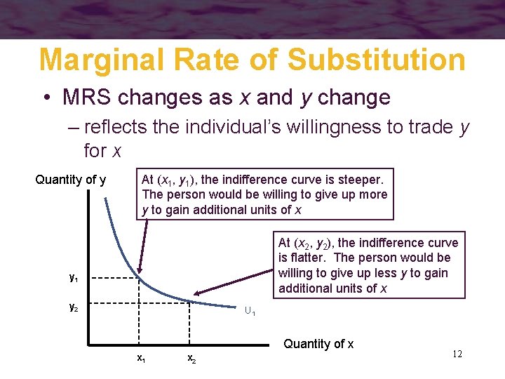
Marginal Rate of Substitution • MRS changes as x and y change – reflects the individual’s willingness to trade y for x Quantity of y At (x 1, y 1), the indifference curve is steeper. The person would be willing to give up more y to gain additional units of x At (x 2, y 2), the indifference curve is flatter. The person would be willing to give up less y to gain additional units of x y 1 y 2 U 1 Quantity of x x 1 x 2 12

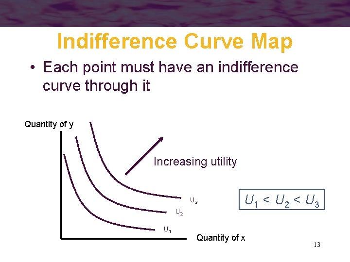
Indifference Curve Map • Each point must have an indifference curve through it Quantity of y Increasing utility U 3 U 2 U 1 < U 2 < U 3 Quantity of x 13

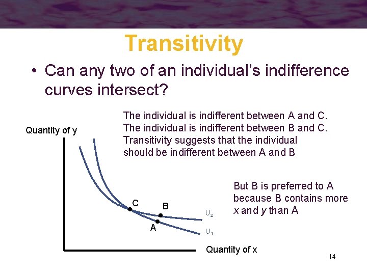
Transitivity • Can any two of an individual’s indifference curves intersect? Quantity of y The individual is indifferent between A and C. The individual is indifferent between B and C. Transitivity suggests that the individual should be indifferent between A and B C B A U 2 But B is preferred to A because B contains more x and y than A U 1 Quantity of x 14

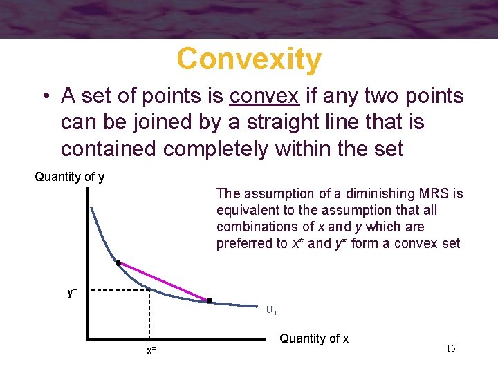
Convexity • A set of points is convex if any two points can be joined by a straight line that is contained completely within the set Quantity of y The assumption of a diminishing MRS is equivalent to the assumption that all combinations of x and y which are preferred to x* and y* form a convex set y* U 1 x* Quantity of x 15

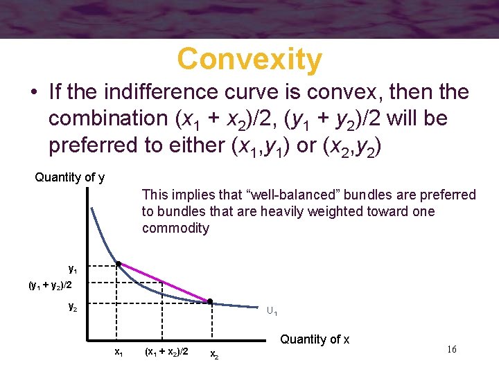
Convexity • If the indifference curve is convex, then the combination (x 1 + x 2)/2, (y 1 + y 2)/2 will be preferred to either (x 1, y 1) or (x 2, y 2) Quantity of y This implies that “well-balanced” bundles are preferred to bundles that are heavily weighted toward one commodity y 1 (y 1 + y 2)/2 y 2 U 1 x 1 (x 1 + x 2)/2 Quantity of x x 2 16

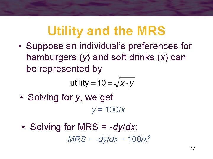
Utility and the MRS • Suppose an individual’s preferences for hamburgers (y) and soft drinks (x) can be represented by • Solving for y, we get y = 100/x • Solving for MRS = -dy/dx: MRS = -dy/dx = 100/x 2 17

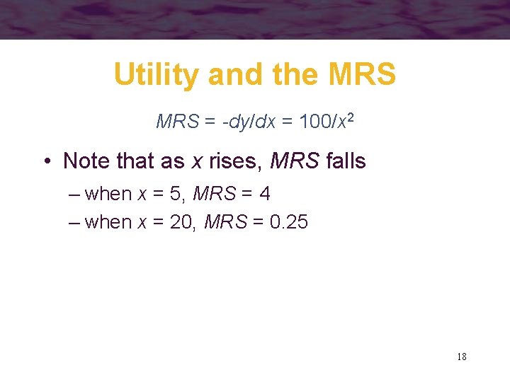
Utility and the MRS = -dy/dx = 100/x 2 • Note that as x rises, MRS falls – when x = 5, MRS = 4 – when x = 20, MRS = 0. 25 18

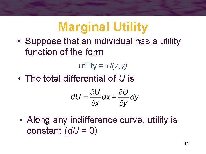
Marginal Utility • Suppose that an individual has a utility function of the form utility = U(x, y) • The total differential of U is • Along any indifference curve, utility is constant (d. U = 0) 19

Deriving the MRS • Therefore, we get: • MRS is the ratio of the marginal utility of x to the marginal utility of y 20

Diminishing Marginal Utility and the MRS • Intuitively, it seems that the assumption of decreasing marginal utility is related to the concept of a diminishing MRS – diminishing MRS requires that the utility function be quasi-concave • this is independent of how utility is measured – diminishing marginal utility depends on how utility is measured • Thus, these two concepts are different 21

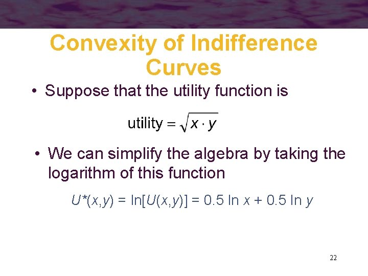
Convexity of Indifference Curves • Suppose that the utility function is • We can simplify the algebra by taking the logarithm of this function U*(x, y) = ln[U(x, y)] = 0. 5 ln x + 0. 5 ln y 22

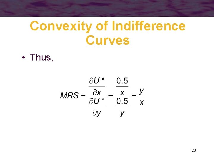
Convexity of Indifference Curves • Thus, 23

Convexity of Indifference Curves • If the utility function is U(x, y) = x + xy + y • There is no advantage to transforming this utility function, so 24

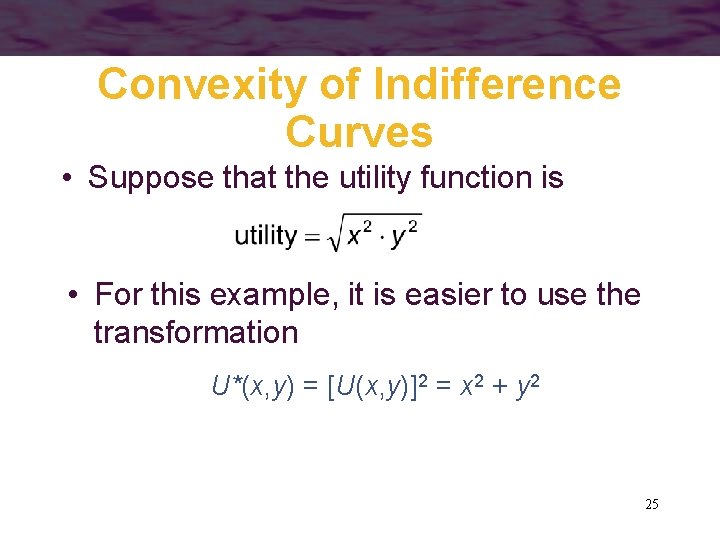
Convexity of Indifference Curves • Suppose that the utility function is • For this example, it is easier to use the transformation U*(x, y) = [U(x, y)]2 = x 2 + y 2 25

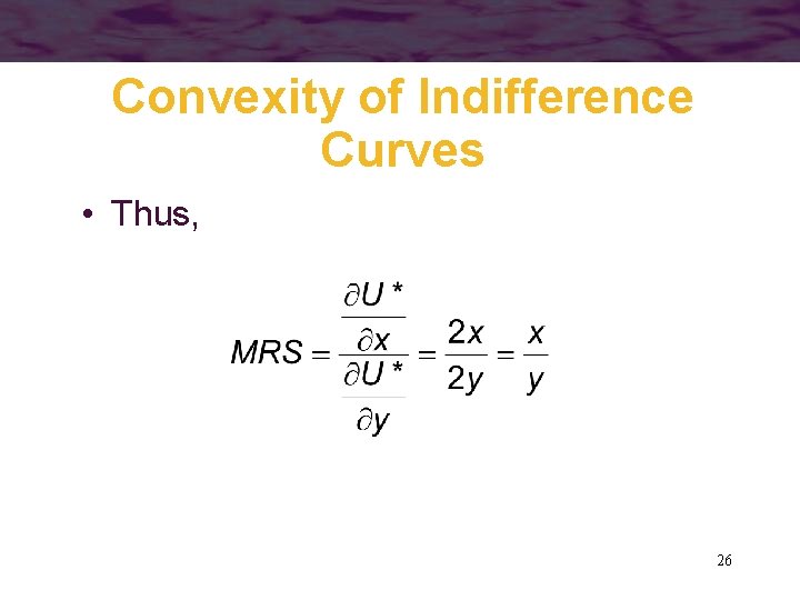
Convexity of Indifference Curves • Thus, 26

Examples of Utility Functions • Cobb-Douglas Utility utility = U(x, y) = x y where and are positive constants – The relative sizes of and indicate the relative importance of the goods 27

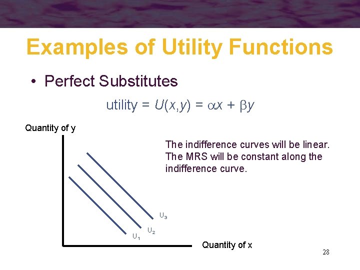
Examples of Utility Functions • Perfect Substitutes utility = U(x, y) = x + y Quantity of y The indifference curves will be linear. The MRS will be constant along the indifference curve. U 3 U 1 U 2 Quantity of x 28

Examples of Utility Functions • Perfect Complements utility = U(x, y) = min ( x, y) Quantity of y The indifference curves will be L-shaped. Only by choosing more of the two goods together can utility be increased. U 3 U 2 U 1 Quantity of x 29

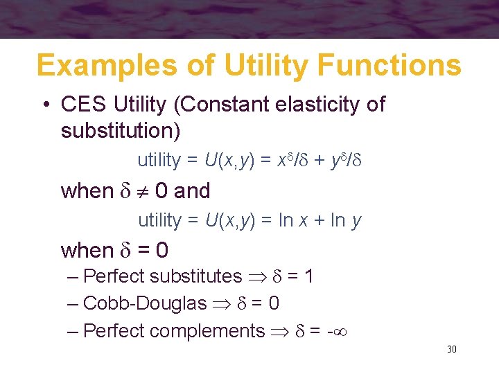
Examples of Utility Functions • CES Utility (Constant elasticity of substitution) utility = U(x, y) = x / + y / when 0 and utility = U(x, y) = ln x + ln y when = 0 – Perfect substitutes = 1 – Cobb-Douglas = 0 – Perfect complements = - 30

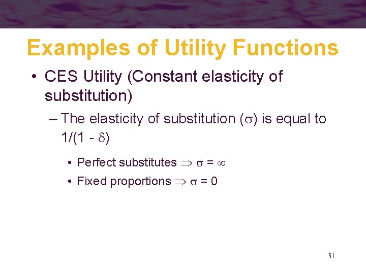
Examples of Utility Functions • CES Utility (Constant elasticity of substitution) – The elasticity of substitution ( ) is equal to 1/(1 - ) • Perfect substitutes = • Fixed proportions = 0 31

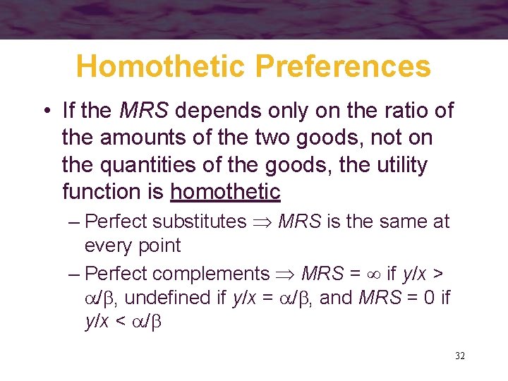
Homothetic Preferences • If the MRS depends only on the ratio of the amounts of the two goods, not on the quantities of the goods, the utility function is homothetic – Perfect substitutes MRS is the same at every point – Perfect complements MRS = if y/x > / , undefined if y/x = / , and MRS = 0 if y/x < / 32

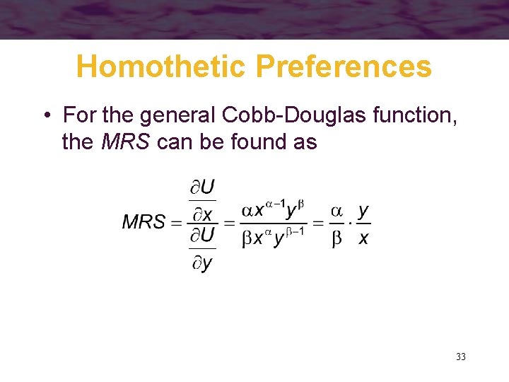
Homothetic Preferences • For the general Cobb-Douglas function, the MRS can be found as 33

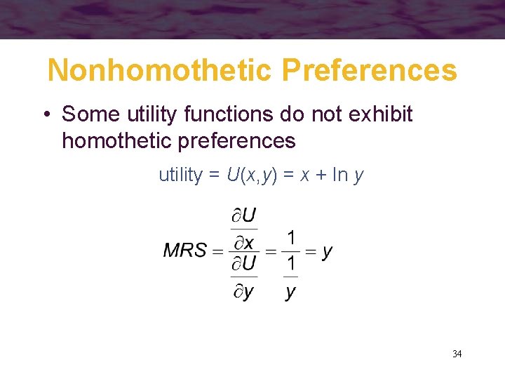
Nonhomothetic Preferences • Some utility functions do not exhibit homothetic preferences utility = U(x, y) = x + ln y 34

The Many-Good Case • Suppose utility is a function of n goods given by utility = U(x 1, x 2, …, xn) • The total differential of U is 35

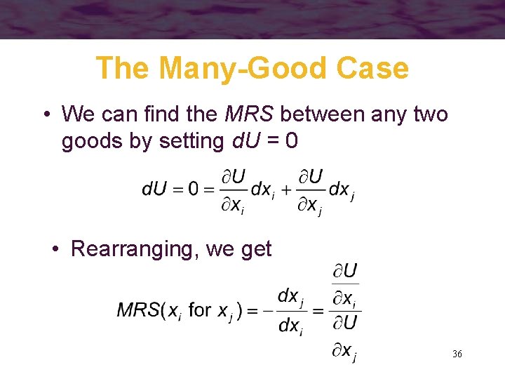
The Many-Good Case • We can find the MRS between any two goods by setting d. U = 0 • Rearranging, we get 36

Multigood Indifference Surfaces • We will define an indifference surface as being the set of points in n dimensions that satisfy the equation U(x 1, x 2, …xn) = k where k is any preassigned constant 37

Multigood Indifference Surfaces • If the utility function is quasi-concave, the set of points for which U k will be convex – all of the points on a line joining any two points on the U = k indifference surface will also have U k 38

Important Points to Note: • If individuals obey certain behavioral postulates, they will be able to rank all commodity bundles – the ranking can be represented by a utility function – in making choices, individuals will act as if they were maximizing this function • Utility functions for two goods can be illustrated by an indifference curve map 39

Important Points to Note: • The negative of the slope of the indifference curve measures the marginal rate of substitution (MRS) – the rate at which an individual would trade an amount of one good (y) for one more unit of another good (x) • MRS decreases as x is substituted for y – individuals prefer some balance in their consumption choices 40

Important Points to Note: • A few simple functional forms can capture important differences in individuals’ preferences for two (or more) goods – Cobb-Douglas function – linear function (perfect substitutes) – fixed proportions function (perfect complements) – CES function • includes the other three as special cases 41

Important Points to Note: • It is a simple matter to generalize from two-good examples to many goods – studying peoples’ choices among many goods can yield many insights – the mathematics of many goods is not especially intuitive, so we will rely on twogood cases to build intuition 42