Chapter 3 MaximumLikelihood Bayesian Parameter Estimation Introduction MaximumLikelihood

Chapter 3: Maximum-Likelihood & Bayesian Parameter Estimation Introduction Maximum-Likelihood Estimation – Example of a Specific Case – The Gaussian Case: unknown and – Bias

n Introduction – Data availability in a Bayesian framework § We could design an optimal classifier if we knew: – P( i) (priors) – P(x | i) (class-conditional densities) Unfortunately, we rarely have this complete information! – Design a classifier from a training sample § No problem with prior estimation § Samples are often too small for class-conditional estimation (large dimension of feature space!) 1

– A priori information about the problem – Normality of P(x | i) ~ N( i, i) § Characterized by 2 parameters – Estimation techniques § Maximum-Likelihood (ML) and the Bayesian estimations § Results are nearly identical, but the approaches are different (they are the same on the limit of infinite number of samples) 1

§ Parameters in ML estimation are fixed but unknown! § Best parameters are obtained by maximizing the probability of obtaining the samples observed § Bayesian methods view the parameters as random variables having some known distribution § In either approach, we use P( i | x) for our classification rule! § We can use estimation for other problems too! 1

n Maximum-Likelihood Estimation § Has good convergence properties as the sample size increases § Simpler than any other alternative techniques – General principle § Assume we have c classes and P(x | j) ~ N( j, j) P(x | j) P (x | j, j) where: 2

§ Use the information provided by the training samples to estimate = ( 1, 2, …, c), each i (i = 1, 2, …, c) is associated with each category § Suppose that D contains n samples, x 1, x 2, …, xn § ML estimate of is, by definition the value that maximizes P(D | ) “It is the value of that best agrees with the actually observed training sample” 2

2

§ Optimal estimation – Let = ( 1, 2, …, p)t and let be the gradient operator – We define l( ) as the log-likelihood function l( ) = ln P(D | ) – New problem statement: determine that maximizes the log-likelihood 2

Set of necessary conditions for an optimum is: l = 0 2

n Example of a specific case: unknown – P(xi | ) ~ N( , ) (Samples are drawn from a multivariate normal population) = therefore: • The ML estimate for must satisfy: 2

• Multiplying by and rearranging, we obtain: Just the arithmetic average of the samples of the training samples! (Exhale now! ) Conclusion: If P(xk | j) (j = 1, 2, …, c) is supposed to be Gaussian in a ddimensional feature space; then we can estimate the vector = ( 1, 2, …, c)t and perform an optimal classification! 2

n ML Estimation: – Gaussian Case: unknown and = ( 1 , 2 ) = ( , 2 ) 2

Summation: Combining (1) and (2), one obtains: 2

n Bias – ML estimate for 2 is biased – An elementary unbiased estimator for is: 2

n ML Problem Statement – Let D = {x 1, x 2, …, xn} P(x 1, …, xn | ) = 1, n. P(xk | ); |D| = n Our goal is to determine (value of that makes this sample the most representative!) 2

= ( 1, 2, …, c) Problem: find such that: 2

Chapter 3: Maximum-Likelihood and Bayesian Parameter Estimation l Bayesian Estimation (BE) l Bayesian Parameter Estimation: Gaussian Case l Bayesian Parameter Estimation: General Estimation l Problems of Dimensionality l Computational Complexity l Component Analysis and Discriminants l Hidden Markov Models

n Bayesian Estimation (Bayesian learning to pattern classification problems) – In MLE was supposed fix – In BE is a random variable – The computation of posterior probabilities P( i | x) lies at the heart of Bayesian classification – Goal: compute P( i | x, D) Given the sample D, Bayes formula can be written 3

n To demonstrate the preceding equation, use: 3

n Bayesian Parameter Estimation: Gaussian Case Goal: Estimate using the a-posteriori density P( | D) The univariate case: P( | D) is the only unknown parameter ( 0 and 0 are known!) 4

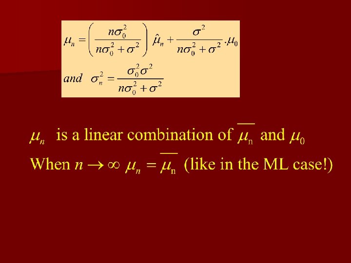
– Reproducing density Identifying (1) and (2) yields: 4

4

– The univariate case P(x | D) § P( | D) computed § P(x | D) remains to be computed! It provides: (Desired class-conditional density P(x | Dj, j)) Therefore: P(x | Dj, j) together with P( j) And using Bayes formula, we obtain the Bayesian classification rule: 4

n Bayesian Parameter Estimation: General Theory – P(x | D) computation can be applied to any situation in which the unknown density can be parametrized: the basic assumptions are: § The form of P(x | ) is assumed known, but the value of is not known exactly § Our knowledge about is assumed to be contained in a known prior density P( ) § The rest of our knowledge is contained in a set D of n random variables x 1, x 2, …, xn that 5 follows P(x)

The basic problem is: “Compute the posterior density P( | D)” then “Derive P(x | D)” Using Bayes formula, we have: And by independence assumption: 5

More cases: Binary Variables n Coin flipping: heads=1, tails=0 n Bernoulli Distribution

Binary variables (2) n. N coin flips: n Binomial Distribution

Binomial distribution

Parameter Estimation ML for Bernoulli Given:

Parameter Estimation (2) n Example: n Prediction: all future tosses will land heads up n Overfitting to D

Beta Distribution n Distribution over .

Bayesian Bernoulli The Beta distribution provides the conjugate prior for the Bernoulli distribution.

Beta Distribution

Prior ∙ Likelihood = Posterior

Properties of the Posterior As the size of the data set, N , increase

Prediction under the Posterior What is the probability that the next coin toss will land heads up?

Multinomial Variables

ML Parameter estimation n Given: n Ensure , use a Lagrange multiplier, ¸.

The Multinomial Distribution

The Dirichlet Distribution Conjugate prior for the multinomial distribution.

Bayesian Multinomial (1)

Bayesian Multinomial (2)

n Problems of Dimensionality – Problems involving 50 or 100 features (binary valued) § Classification accuracy depends upon the dimensionality and the amount of training data § Case of two classes multivariate normal with the same covariance 7

§ If features are independent then: § Most useful features are the ones for which the difference between the means is large relative to the standard deviation § It has frequently been observed in practice that, beyond a certain point, the inclusion of additional features leads to worse rather than better performance: we have the wrong model ! 7

7 7

n Computational Complexity – Our design methodology is affected by the computational difficulty § “big oh” notation f(x) = O(h(x)) “big oh of h(x)” If: (An upper bound on f(x) grows no worse than h(x) for sufficiently large x!) f(x) = 2+3 x+4 x 2 g(x) = x 2 7

– “big oh” is not unique! f(x) = O(x 2); f(x) = O(x 3); f(x) = O(x 4) § “big theta” notation f(x) = (h(x)) If: f(x) = (x 2) but f(x) (x 3) 7

– Complexity of the ML Estimation § Gaussian priors in d dimensions classifier with n training samples for each of c classes § For each category, we have to compute the discriminant function Total = O(d 2. . n) Total for c classes = O(cd 2. n) O(d 2. n) 7

n Component Analysis and Discriminants – Combine features in order to reduce the dimension of the feature space – Linear combinations are simple to compute and tractable – Project high dimensional data onto a lower dimensional space – Two classical approaches for finding “optimal” linear transformation § PCA (Principal Component Analysis) “Projection that best represents the data in a least- square sense” § MDA (Multiple Discriminant Analysis) “Projection that best separates the data in a least-squares sense” 8

Expectation Maximization n Learning parameters governing a distribution from training points with missing values A generalization of MLE Missing features Consider Improved estimate Best estimate so far Marginalized w/respect to current estimate

EM Algorithm

EM example: Mixtures of Gaussians Pick estimates of Plug them here Use the result to solve these Use the new estimate to go back to the E-step …

Gaussian Mixture Example: Start

After first iteration

After 2 nd iteration

After 3 rd iteration

After 4 th iteration

After 5 th iteration

After 6 th iteration

After 20 th iteration

n Hidden Markov Models: – Markov Chains – Goal: make a sequence of decisions § Processes that unfold in time, states at time t are influenced by a state at time t-1 § Applications: speech recognition, gesture recognition, parts of speech tagging and DNA sequencing, § Any temporal process without memory T = { (1), (2), (3), …, (T)} sequence of states 10 We might have 6 = { 1, 4, 2, 1, 4}

– First-order Markov models § Our productions of any sequence is described by the transition probabilities P( j(t + 1) | i (t)) = aij 10

10

= (aij, T) P( T | ) = a 14. a 42. a 21. a 14. P( (1) = i) Example: speech recognition “production of spoken words” Production of the word: “pattern” represented by phonemes /p/ /a/ /tt/ /er/ /n/ // ( // = silent state) Transitions from /p/ to /a/, /a/ to /tt/, /tt/ to er/, /er/ to /n/ and /n/ to a silent state 10

HMMs