Chapter 3 Linear Programming Modeling Applications 2007 Pearson

Chapter 3: Linear Programming Modeling Applications © 2007 Pearson Education

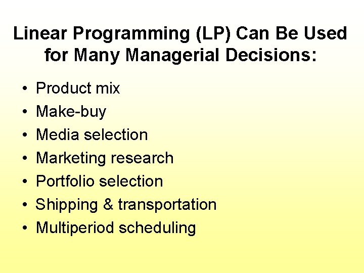
Linear Programming (LP) Can Be Used for Many Managerial Decisions: • • Product mix Make-buy Media selection Marketing research Portfolio selection Shipping & transportation Multiperiod scheduling

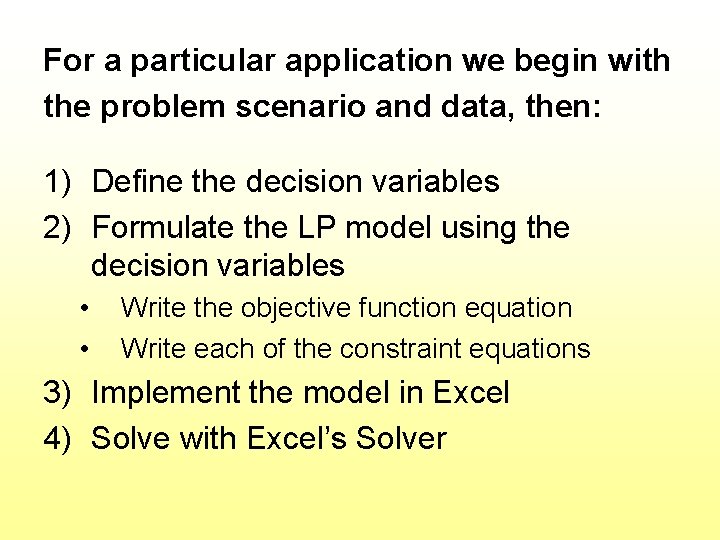
For a particular application we begin with the problem scenario and data, then: 1) Define the decision variables 2) Formulate the LP model using the decision variables • • Write the objective function equation Write each of the constraint equations 3) Implement the model in Excel 4) Solve with Excel’s Solver

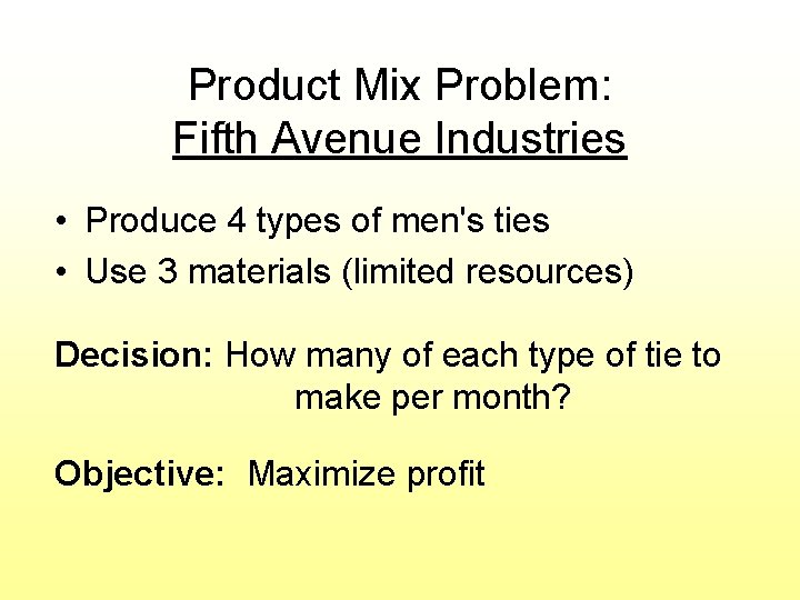
Product Mix Problem: Fifth Avenue Industries • Produce 4 types of men's ties • Use 3 materials (limited resources) Decision: How many of each type of tie to make per month? Objective: Maximize profit

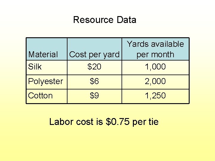
Resource Data Material Silk Yards available Cost per yard per month $20 1, 000 Polyester $6 2, 000 Cotton $9 1, 250 Labor cost is $0. 75 per tie

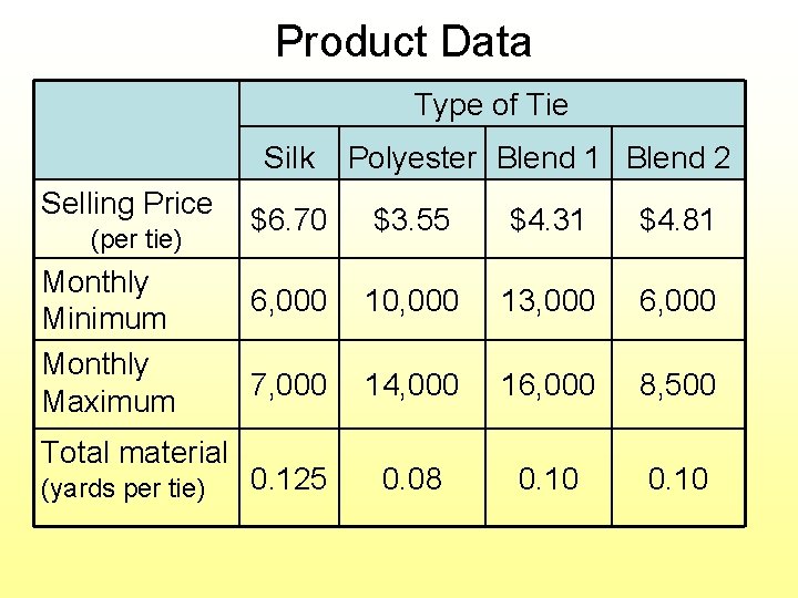
Product Data Type of Tie Silk Selling Price (per tie) Monthly Minimum Monthly Maximum Total material (yards per tie) Polyester Blend 1 Blend 2 $6. 70 $3. 55 $4. 31 $4. 81 6, 000 10, 000 13, 000 6, 000 7, 000 14, 000 16, 000 8, 500 0. 125 0. 08 0. 10

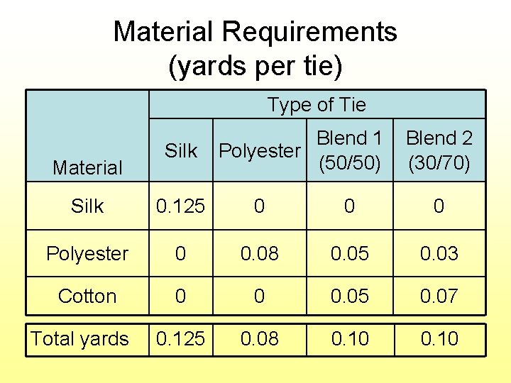
Material Requirements (yards per tie) Type of Tie Material Silk Blend 1 Polyester (50/50) Blend 2 (30/70) Silk 0. 125 0 0 0 Polyester 0 0. 08 0. 05 0. 03 Cotton 0 0 0. 05 0. 07 0. 125 0. 08 0. 10 Total yards

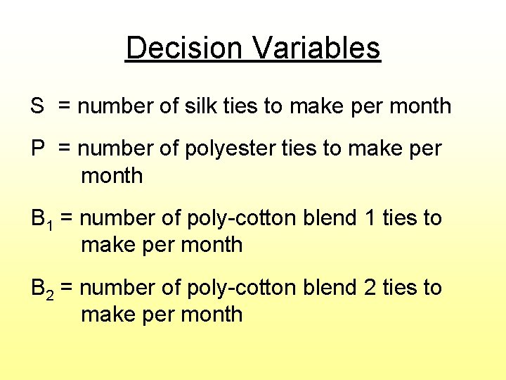
Decision Variables S = number of silk ties to make per month P = number of polyester ties to make per month B 1 = number of poly-cotton blend 1 ties to make per month B 2 = number of poly-cotton blend 2 ties to make per month

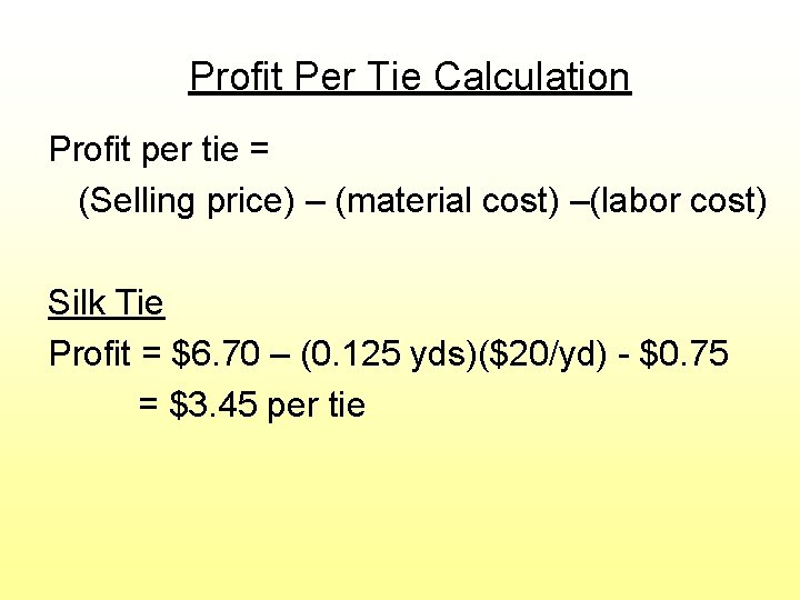
Profit Per Tie Calculation Profit per tie = (Selling price) – (material cost) –(labor cost) Silk Tie Profit = $6. 70 – (0. 125 yds)($20/yd) - $0. 75 = $3. 45 per tie

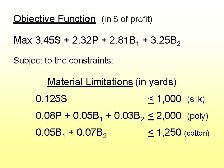
Objective Function (in $ of profit) Max 3. 45 S + 2. 32 P + 2. 81 B 1 + 3. 25 B 2 Subject to the constraints: Material Limitations (in yards) 0. 125 S < 1, 000 (silk) 0. 08 P + 0. 05 B 1 + 0. 03 B 2 < 2, 000 (poly) 0. 05 B 1 + 0. 07 B 2 < 1, 250 (cotton)

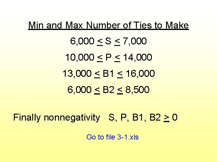
Min and Max Number of Ties to Make 6, 000 < S < 7, 000 10, 000 < P < 14, 000 13, 000 < B 1 < 16, 000 < B 2 < 8, 500 Finally nonnegativity S, P, B 1, B 2 > 0 Go to file 3 -1. xls

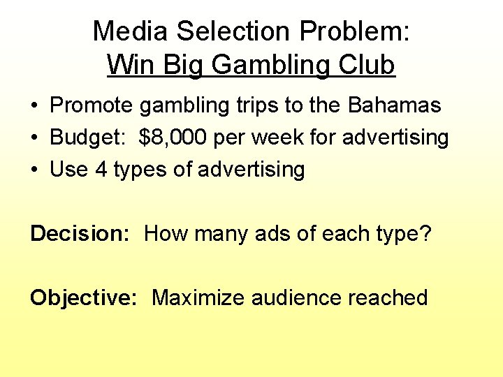
Media Selection Problem: Win Big Gambling Club • Promote gambling trips to the Bahamas • Budget: $8, 000 per week for advertising • Use 4 types of advertising Decision: How many ads of each type? Objective: Maximize audience reached

Data TV Spot Advertising Options Radio Newspaper (prime time) Radio (afternoon) Audience Reached (per ad) 5, 000 8, 500 2, 400 2, 800 Cost (per ad) $800 $925 $290 $380 Max Ads Per week 12 5 25 20

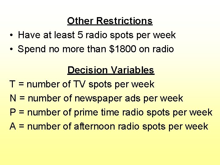
Other Restrictions • Have at least 5 radio spots per week • Spend no more than $1800 on radio Decision Variables T = number of TV spots per week N = number of newspaper ads per week P = number of prime time radio spots per week A = number of afternoon radio spots per week

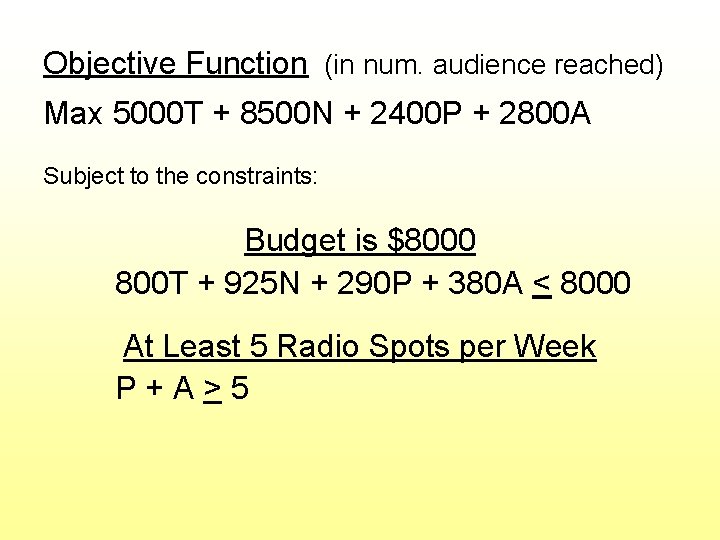
Objective Function (in num. audience reached) Max 5000 T + 8500 N + 2400 P + 2800 A Subject to the constraints: Budget is $8000 800 T + 925 N + 290 P + 380 A < 8000 At Least 5 Radio Spots per Week P+A>5

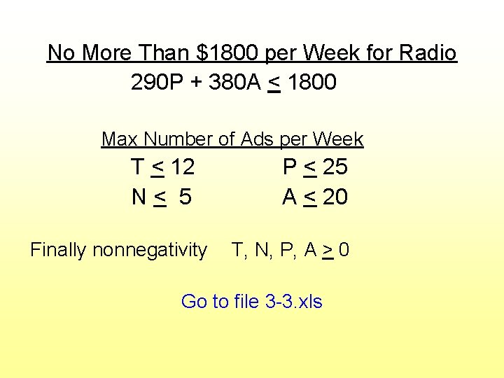
No More Than $1800 per Week for Radio 290 P + 380 A < 1800 Max Number of Ads per Week T < 12 N< 5 Finally nonnegativity P < 25 A < 20 T, N, P, A > 0 Go to file 3 -3. xls

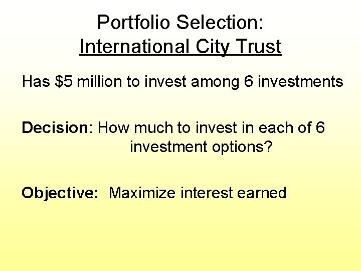
Portfolio Selection: International City Trust Has $5 million to invest among 6 investments Decision: How much to invest in each of 6 investment options? Objective: Maximize interest earned

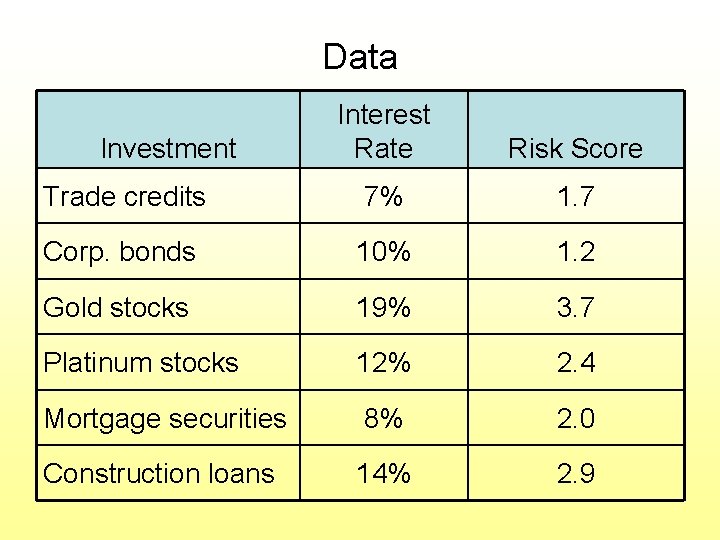
Data Interest Rate Risk Score Trade credits 7% 1. 7 Corp. bonds 10% 1. 2 Gold stocks 19% 3. 7 Platinum stocks 12% 2. 4 Mortgage securities 8% 2. 0 Construction loans 14% 2. 9 Investment

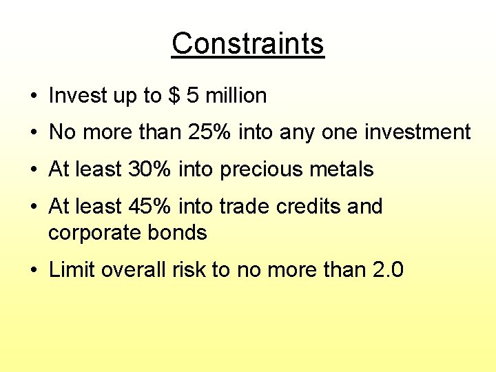
Constraints • Invest up to $ 5 million • No more than 25% into any one investment • At least 30% into precious metals • At least 45% into trade credits and corporate bonds • Limit overall risk to no more than 2. 0

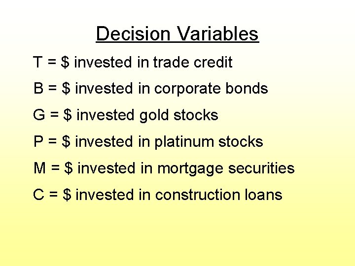
Decision Variables T = $ invested in trade credit B = $ invested in corporate bonds G = $ invested gold stocks P = $ invested in platinum stocks M = $ invested in mortgage securities C = $ invested in construction loans

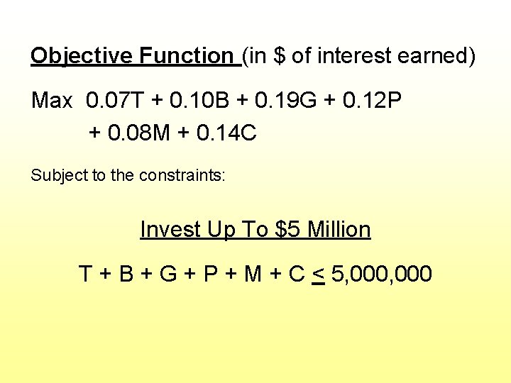
Objective Function (in $ of interest earned) Max 0. 07 T + 0. 10 B + 0. 19 G + 0. 12 P + 0. 08 M + 0. 14 C Subject to the constraints: Invest Up To $5 Million T + B + G + P + M + C < 5, 000

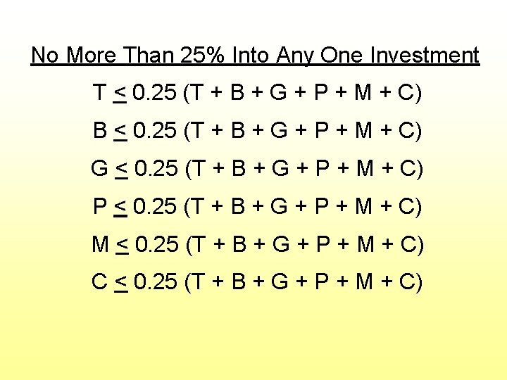
No More Than 25% Into Any One Investment T < 0. 25 (T + B + G + P + M + C) B < 0. 25 (T + B + G + P + M + C) G < 0. 25 (T + B + G + P + M + C) P < 0. 25 (T + B + G + P + M + C) M < 0. 25 (T + B + G + P + M + C) C < 0. 25 (T + B + G + P + M + C)

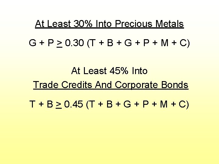
At Least 30% Into Precious Metals G + P > 0. 30 (T + B + G + P + M + C) At Least 45% Into Trade Credits And Corporate Bonds T + B > 0. 45 (T + B + G + P + M + C)

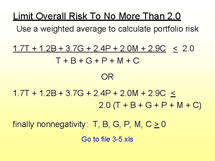
Limit Overall Risk To No More Than 2. 0 Use a weighted average to calculate portfolio risk 1. 7 T + 1. 2 B + 3. 7 G + 2. 4 P + 2. 0 M + 2. 9 C < 2. 0 T+B+G+P+M+C OR 1. 7 T + 1. 2 B + 3. 7 G + 2. 4 P + 2. 0 M + 2. 9 C < 2. 0 (T + B + G + P + M + C) finally nonnegativity: T, B, G, P, M, C > 0 Go to file 3 -5. xls

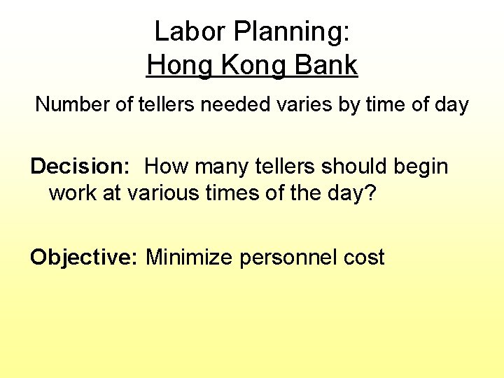
Labor Planning: Hong Kong Bank Number of tellers needed varies by time of day Decision: How many tellers should begin work at various times of the day? Objective: Minimize personnel cost

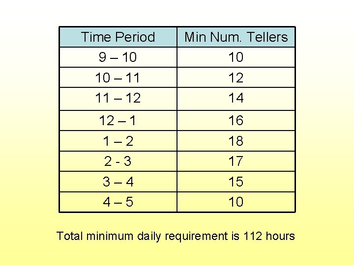
Time Period 9 – 10 10 – 11 11 – 12 Min Num. Tellers 10 12 14 12 – 1 1– 2 2 -3 3– 4 4– 5 16 18 17 15 10 Total minimum daily requirement is 112 hours

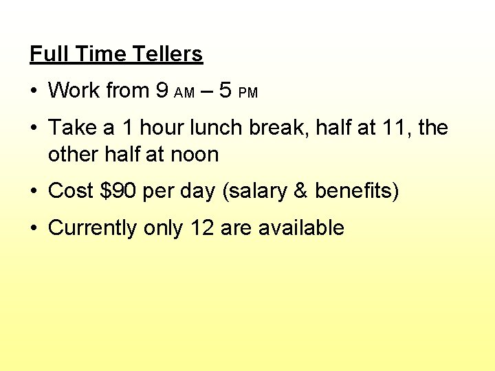
Full Time Tellers • Work from 9 AM – 5 PM • Take a 1 hour lunch break, half at 11, the other half at noon • Cost $90 per day (salary & benefits) • Currently only 12 are available

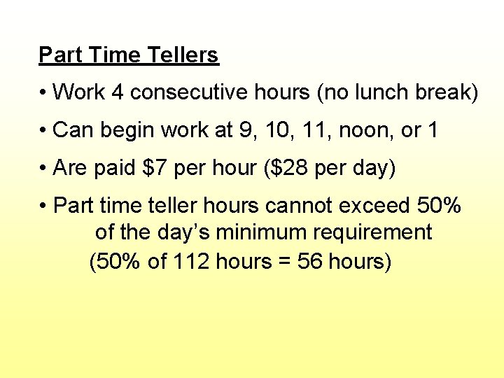
Part Time Tellers • Work 4 consecutive hours (no lunch break) • Can begin work at 9, 10, 11, noon, or 1 • Are paid $7 per hour ($28 per day) • Part time teller hours cannot exceed 50% of the day’s minimum requirement (50% of 112 hours = 56 hours)

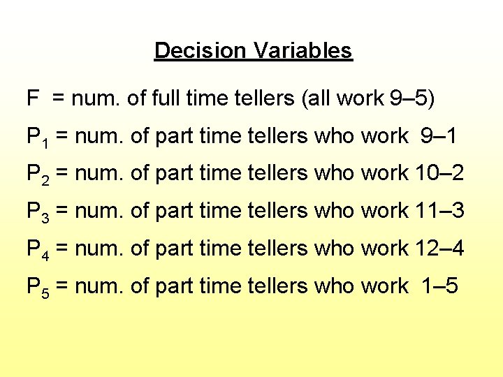
Decision Variables F = num. of full time tellers (all work 9– 5) P 1 = num. of part time tellers who work 9– 1 P 2 = num. of part time tellers who work 10– 2 P 3 = num. of part time tellers who work 11– 3 P 4 = num. of part time tellers who work 12– 4 P 5 = num. of part time tellers who work 1– 5

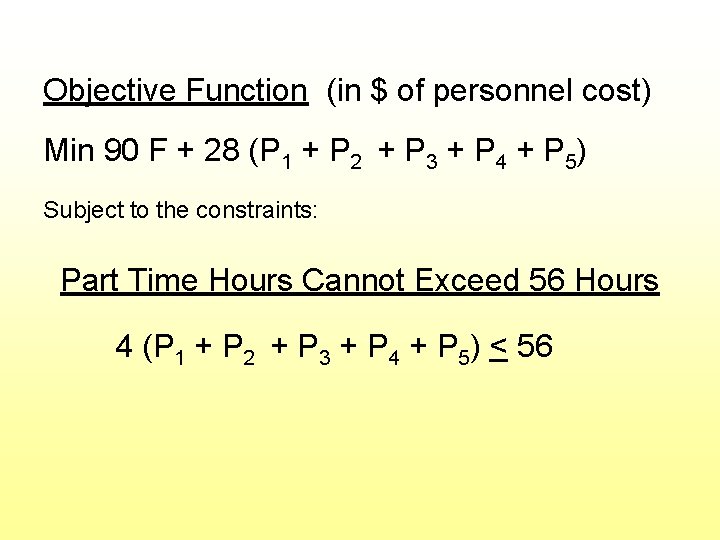
Objective Function (in $ of personnel cost) Min 90 F + 28 (P 1 + P 2 + P 3 + P 4 + P 5) Subject to the constraints: Part Time Hours Cannot Exceed 56 Hours 4 (P 1 + P 2 + P 3 + P 4 + P 5) < 56

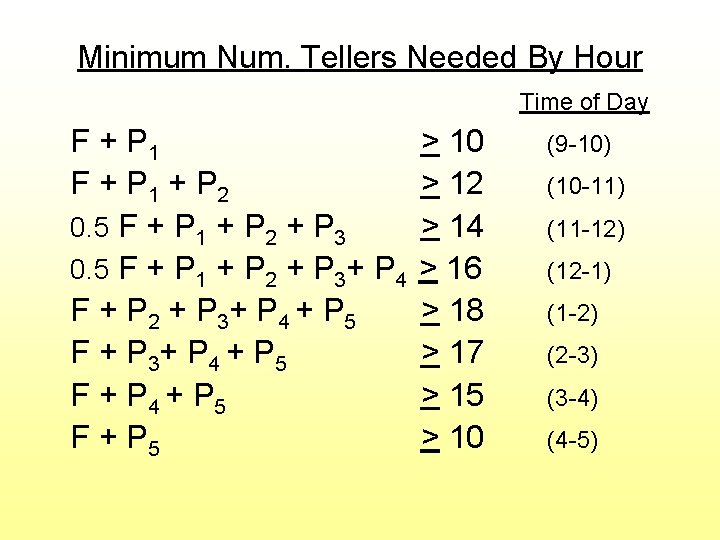
Minimum Num. Tellers Needed By Hour Time of Day F + P 1 + P 2 0. 5 F + P 1 + P 2 + P 3+ P 4 F + P 2 + P 3+ P 4 + P 5 F + P 5 > 10 > 12 > 14 > 16 > 18 > 17 > 15 > 10 (9 -10) (10 -11) (11 -12) (12 -1) (1 -2) (2 -3) (3 -4) (4 -5)

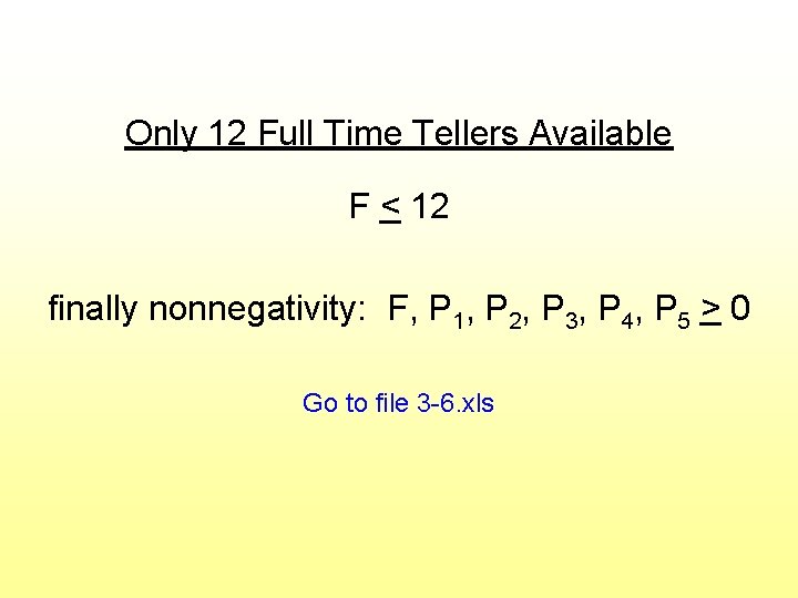
Only 12 Full Time Tellers Available F < 12 finally nonnegativity: F, P 1, P 2, P 3, P 4, P 5 > 0 Go to file 3 -6. xls

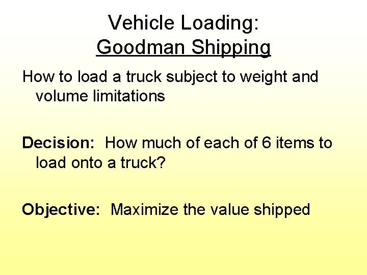
Vehicle Loading: Goodman Shipping How to load a truck subject to weight and volume limitations Decision: How much of each of 6 items to load onto a truck? Objective: Maximize the value shipped

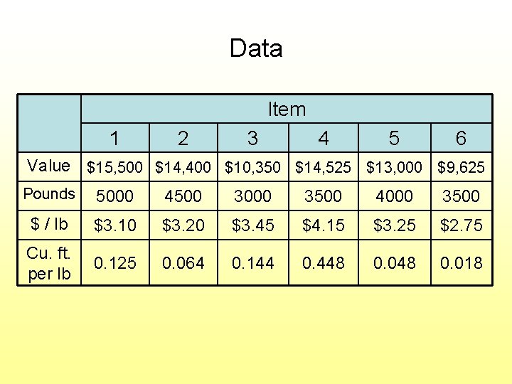
Data Item 1 2 3 4 5 6 Value $15, 500 $14, 400 $10, 350 $14, 525 $13, 000 $9, 625 Pounds 5000 4500 3000 3500 4000 3500 $ / lb $3. 10 $3. 20 $3. 45 $4. 15 $3. 25 $2. 75 Cu. ft. per lb 0. 125 0. 064 0. 144 0. 448 0. 018

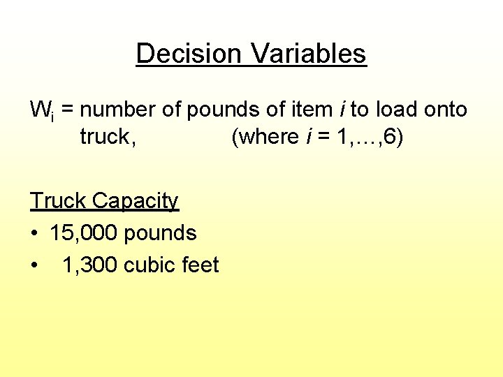
Decision Variables Wi = number of pounds of item i to load onto truck, (where i = 1, …, 6) Truck Capacity • 15, 000 pounds • 1, 300 cubic feet

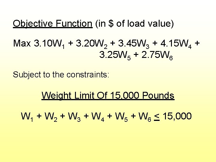
Objective Function (in $ of load value) Max 3. 10 W 1 + 3. 20 W 2 + 3. 45 W 3 + 4. 15 W 4 + 3. 25 W 5 + 2. 75 W 6 Subject to the constraints: Weight Limit Of 15, 000 Pounds W 1 + W 2 + W 3 + W 4 + W 5 + W 6 < 15, 000

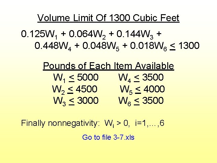
Volume Limit Of 1300 Cubic Feet 0. 125 W 1 + 0. 064 W 2 + 0. 144 W 3 + 0. 448 W 4 + 0. 048 W 5 + 0. 018 W 6 < 1300 Pounds of Each Item Available W 1 < 5000 W 4 < 3500 W 2 < 4500 W 5 < 4000 W 3 < 3000 W 6 < 3500 Finally nonnegativity: Wi > 0, i=1, …, 6 Go to file 3 -7. xls

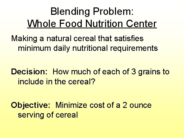
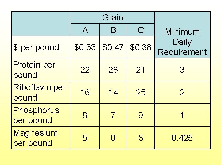
Blending Problem: Whole Food Nutrition Center Making a natural cereal that satisfies minimum daily nutritional requirements Decision: How much of each of 3 grains to include in the cereal? Objective: Minimize cost of a 2 ounce serving of cereal

$ per pound Protein per pound Riboflavin per pound Phosphorus per pound Magnesium per pound A Grain B C 22 28 21 3 16 14 25 2 8 7 9 1 5 0 6 0. 425 Minimum Daily $0. 33 $0. 47 $0. 38 Requirement

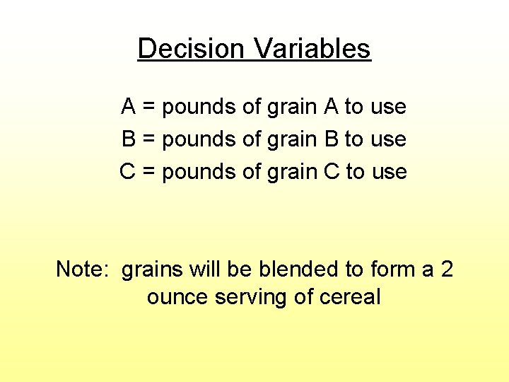
Decision Variables A = pounds of grain A to use B = pounds of grain B to use C = pounds of grain C to use Note: grains will be blended to form a 2 ounce serving of cereal

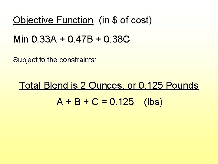
Objective Function (in $ of cost) Min 0. 33 A + 0. 47 B + 0. 38 C Subject to the constraints: Total Blend is 2 Ounces, or 0. 125 Pounds A + B + C = 0. 125 (lbs)

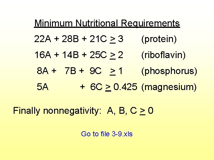
Minimum Nutritional Requirements 22 A + 28 B + 21 C > 3 (protein) 16 A + 14 B + 25 C > 2 (riboflavin) 8 A + 7 B + 9 C > 1 (phosphorus) 5 A + 6 C > 0. 425 (magnesium) Finally nonnegativity: A, B, C > 0 Go to file 3 -9. xls

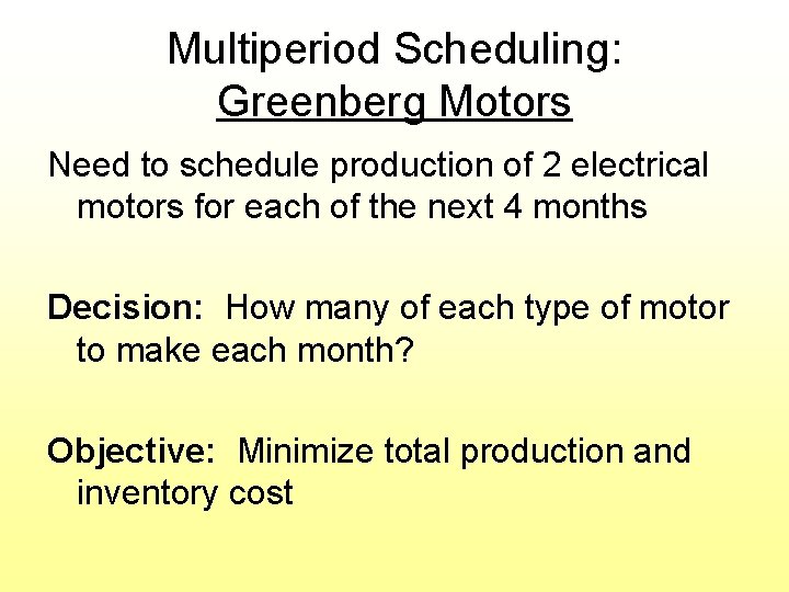
Multiperiod Scheduling: Greenberg Motors Need to schedule production of 2 electrical motors for each of the next 4 months Decision: How many of each type of motor to make each month? Objective: Minimize total production and inventory cost

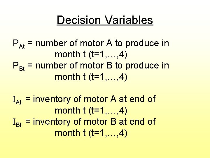
Decision Variables PAt = number of motor A to produce in month t (t=1, …, 4) PBt = number of motor B to produce in month t (t=1, …, 4) IAt = inventory of motor A at end of month t (t=1, …, 4) IBt = inventory of motor B at end of month t (t=1, …, 4)

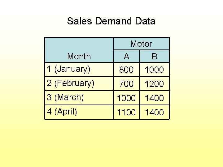
Sales Demand Data Motor A B Month 1 (January) 800 1000 2 (February) 700 1200 3 (March) 1000 1400 4 (April) 1100 1400

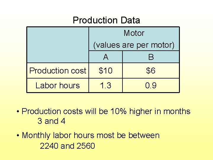
Production Data Motor (values are per motor) A B Production cost $10 $6 Labor hours 1. 3 0. 9 • Production costs will be 10% higher in months 3 and 4 • Monthly labor hours most be between 2240 and 2560

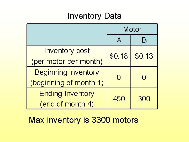
Inventory Data Motor A B Inventory cost $0. 18 $0. 13 (per motor per month) Beginning inventory 0 0 (beginning of month 1) Ending Inventory 450 300 (end of month 4) Max inventory is 3300 motors

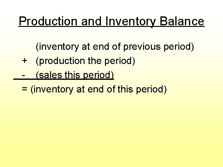
Production and Inventory Balance (inventory at end of previous period) + (production the period) - (sales this period) = (inventory at end of this period)

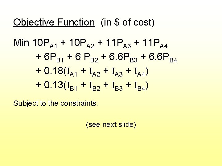
Objective Function (in $ of cost) Min 10 PA 1 + 10 PA 2 + 11 PA 3 + 11 PA 4 + 6 PB 1 + 6 PB 2 + 6. 6 PB 3 + 6. 6 PB 4 + 0. 18(IA 1 + IA 2 + IA 3 + IA 4) + 0. 13(IB 1 + IB 2 + IB 3 + IB 4) Subject to the constraints: (see next slide)

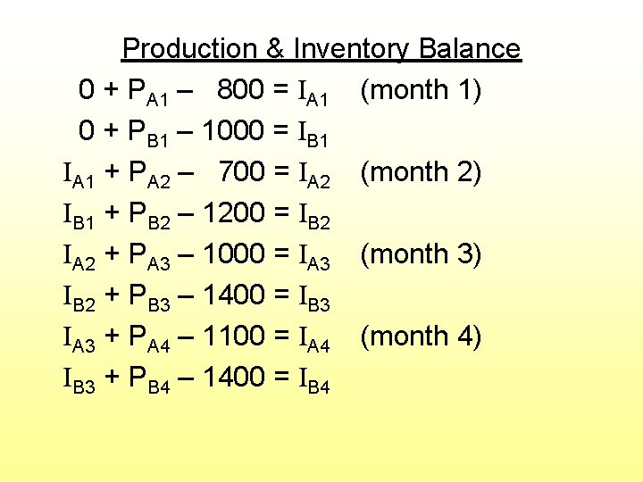
Production & Inventory Balance 0 + PA 1 – 800 = IA 1 (month 1) 0 + PB 1 – 1000 = IB 1 IA 1 + PA 2 – 700 = IA 2 (month 2) IB 1 + PB 2 – 1200 = IB 2 IA 2 + PA 3 – 1000 = IA 3 (month 3) IB 2 + PB 3 – 1400 = IB 3 IA 3 + PA 4 – 1100 = IA 4 (month 4) IB 3 + PB 4 – 1400 = IB 4

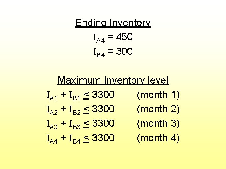
Ending Inventory IA 4 = 450 IB 4 = 300 Maximum Inventory level IA 1 + IB 1 < 3300 (month 1) IA 2 + IB 2 < 3300 (month 2) IA 3 + IB 3 < 3300 (month 3) IA 4 + IB 4 < 3300 (month 4)

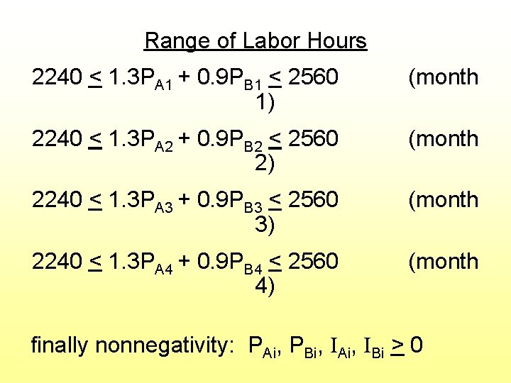
Range of Labor Hours 2240 < 1. 3 PA 1 + 0. 9 PB 1 < 2560 1) (month 2240 < 1. 3 PA 2 + 0. 9 PB 2 < 2560 2) (month 2240 < 1. 3 PA 3 + 0. 9 PB 3 < 2560 3) (month 2240 < 1. 3 PA 4 + 0. 9 PB 4 < 2560 4) (month finally nonnegativity: PAi, PBi, IAi, IBi > 0