Chapter 3 Linear Programming Methods Introduction 1 Whereas

高等作業研究(一) Chapter 3 Linear Programming Methods

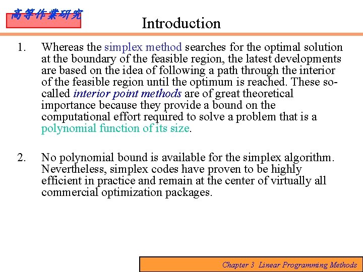
高等作業研究 Introduction 1. Whereas the simplex method searches for the optimal solution at the boundary of the feasible region, the latest developments are based on the idea of following a path through the interior of the feasible region until the optimum is reached. These socalled interior point methods are of great theoretical importance because they provide a bound on the computational effort required to solve a problem that is a polynomial function of its size. 2. No polynomial bound is available for the simplex algorithm. Nevertheless, simplex codes have proven to be highly efficient in practice and remain at the center of virtually all commercial optimization packages. Chapter 3 Linear Programming Methods

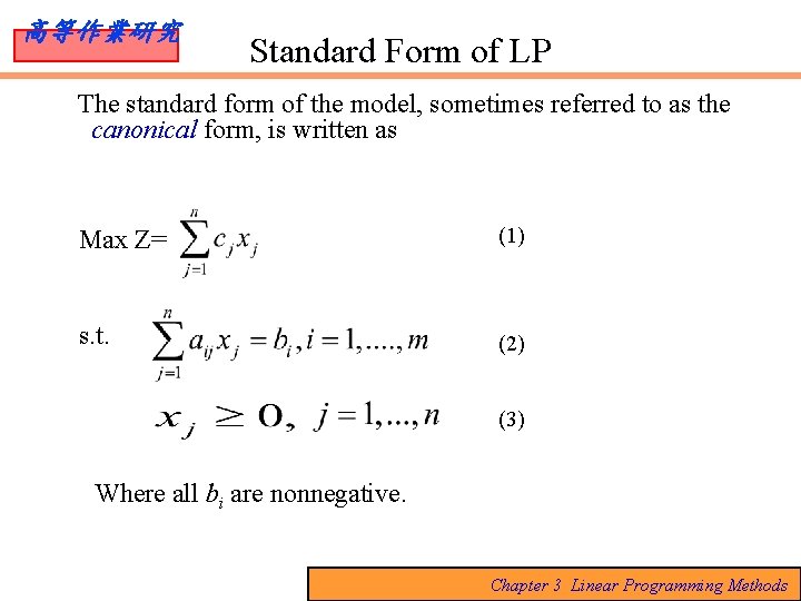
高等作業研究 Standard Form of LP The standard form of the model, sometimes referred to as the canonical form, is written as Max Z= (1) s. t. (2) (3) Where all bi are nonnegative. Chapter 3 Linear Programming Methods

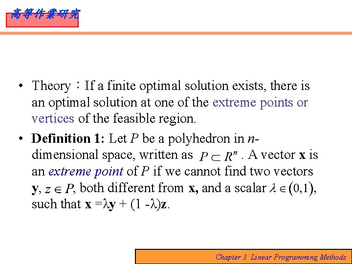
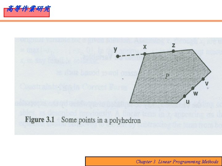
高等作業研究 • Theory：If a finite optimal solution exists, there is an optimal solution at one of the extreme points or vertices of the feasible region. • Definition 1: Let P be a polyhedron in ndimensional space, written as. A vector x is an extreme point of P if we cannot find two vectors y, , both different from x, and a scalar such that x =λy + (1 -λ)z. Chapter 3 Linear Programming Methods

高等作業研究 Chapter 3 Linear Programming Methods

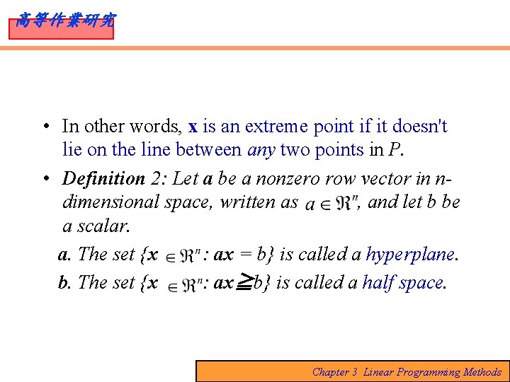
高等作業研究 • In other words, x is an extreme point if it doesn't lie on the line between any two points in P. • Definition 2: Let a be a nonzero row vector in ndimensional space, written as , and let b be a scalar. a. The set {x : ax = b} is called a hyperplane. b. The set {x : ax≧b} is called a half space. Chapter 3 Linear Programming Methods

高等作業研究 • Note that a hyperplane is the boundary of a corresponding halfspace. For a polyhedron in n-dimensional space, an extreme point is the intersection of n non-coplanar hyperplanes. (If more than n hyperplanes are intersected, the extreme point is degenerated. ) • For the linear programming problem defined by Equations (1) to (3), some of these hyperplanes will be of the form = 0. Chapter 3 Linear Programming Methods

高等作業研究 PREPARING THE MODEL • The objective must be to maximize. • The objective function must be linear in the variables and must not contain any constant terms. • All variables must be restricted to be nonnegative. • Each constraint must be written as a linear equation with the variables on the left of the equal sign and a positive constant on the right. Chapter 3 Linear Programming Methods

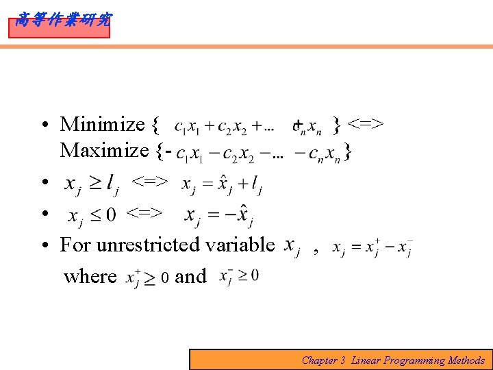
高等作業研究 • Minimize { Maximize { • <=> • For unrestricted variable where 0 and } <=> } , Chapter 3 Linear Programming Methods

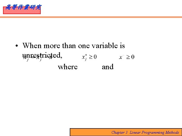
高等作業研究 • When more than one variable is unrestricted, where and Chapter 3 Linear Programming Methods

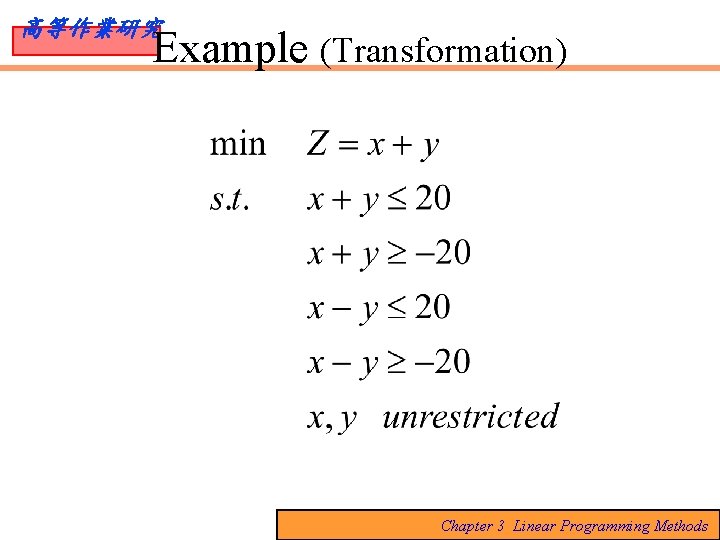
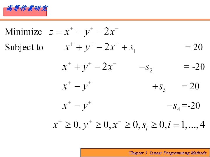
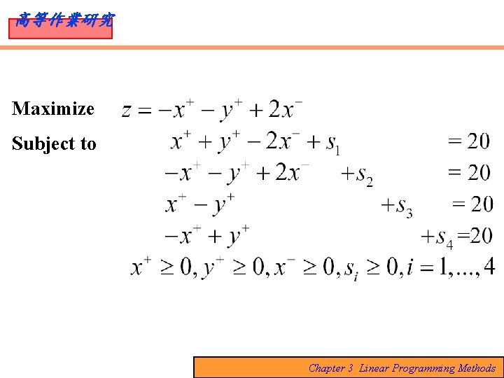
高等作業研究 Example (Transformation) Chapter 3 Linear Programming Methods

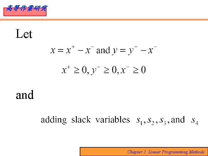
高等作業研究 Let and Chapter 3 Linear Programming Methods

高等作業研究 Chapter 3 Linear Programming Methods

高等作業研究 Maximize Subject to Chapter 3 Linear Programming Methods

高等作業研究 GEOMETRIC PROPERTIES OF LPs When solving two-dimensional problems graphically, we saw that solutions were always found at extreme points of the feasible region. These solutions are called basic solutions. In a problem with n variables and m constraints, a basic solution is determined by identifying m variables as basic, setting the remaining n - m (nonbasic) variables equal to zero, and solving the resultant set of simultaneous equations. Chapter 3 Linear Programming Methods

高等作業研究 In order for these equations to have a unique solution and hence correspond to an extreme point, care must be taken in choosing which variables to make basic. Chapter 3 Linear Programming Methods

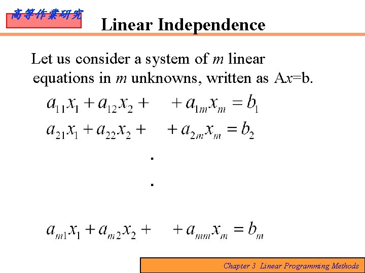
高等作業研究 Linear Independence Let us consider a system of m linear equations in m unknowns, written as Ax=b. Chapter 3 Linear Programming Methods

高等作業研究 For this system to have a unique solution, the matrix A must be invertible or nonsingular— that is, there must exist another m × m matrix B such that AB = BA = I, where I is the m x m identity matrix. Such a matrix B is called the inverse of A and is unique. It is denoted by. Chapter 3 Linear Programming Methods

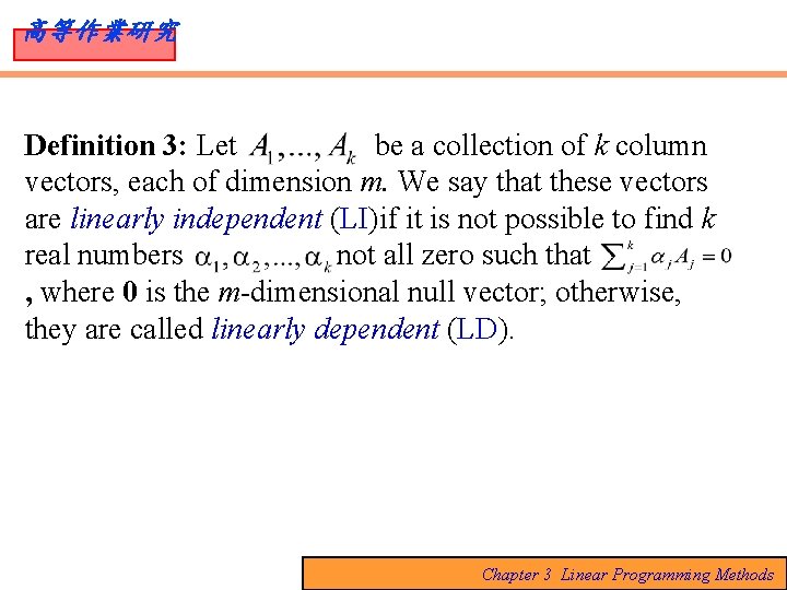
高等作業研究 Definition 3: Let be a collection of k column vectors, each of dimension m. We say that these vectors are linearly independent (LI)if it is not possible to find k real numbers not all zero such that , where 0 is the m-dimensional null vector; otherwise, they are called linearly dependent (LD). Chapter 3 Linear Programming Methods

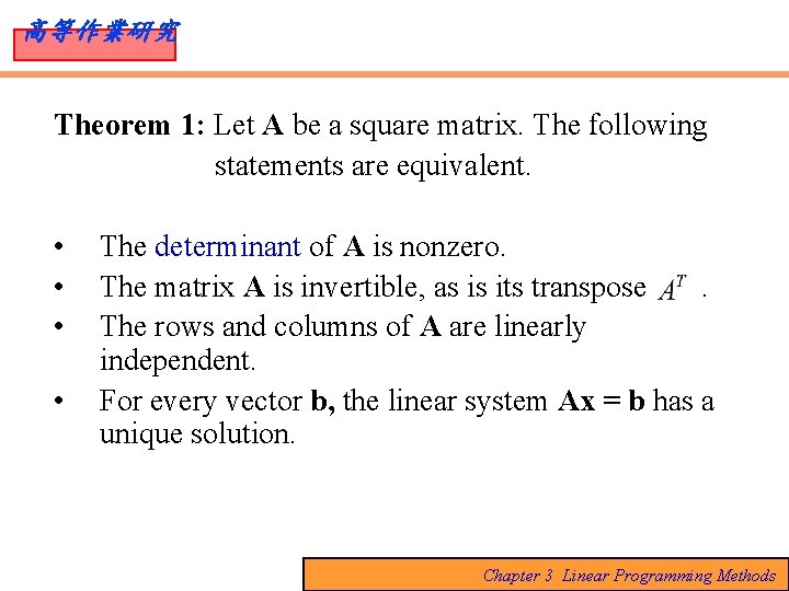
高等作業研究 Theorem 1: Let A be a square matrix. The following statements are equivalent. • • The determinant of A is nonzero. The matrix A is invertible, as is its transpose. The rows and columns of A are linearly independent. For every vector b, the linear system Ax = b has a unique solution. Chapter 3 Linear Programming Methods

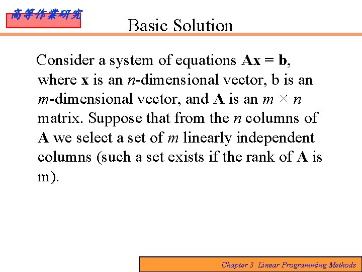
高等作業研究 Basic Solution Consider a system of equations Ax = b, where x is an n-dimensional vector, b is an m-dimensional vector, and A is an m × n matrix. Suppose that from the n columns of A we select a set of m linearly independent columns (such a set exists if the rank of A is m). Chapter 3 Linear Programming Methods

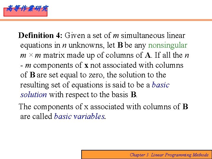
高等作業研究 Definition 4: Given a set of m simultaneous linear equations in n unknowns, let B be any nonsingular m × m matrix made up of columns of A. If all the n - m components of x not associated with columns of B are set equal to zero, the solution to the resulting set of equations is said to be a basic solution with respect to the basis B. The components of x associated with columns of B are called basic variables. Chapter 3 Linear Programming Methods

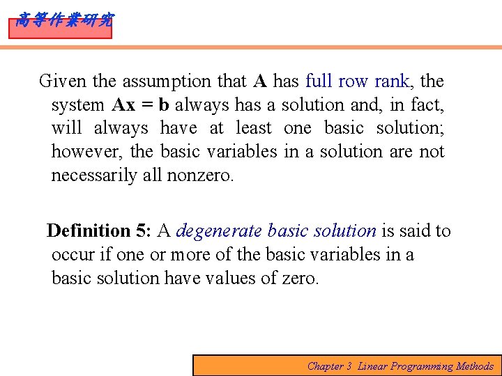
高等作業研究 Given the assumption that A has full row rank, the system Ax = b always has a solution and, in fact, will always have at least one basic solution; however, the basic variables in a solution are not necessarily all nonzero. Definition 5: A degenerate basic solution is said to occur if one or more of the basic variables in a basic solution have values of zero. Chapter 3 Linear Programming Methods

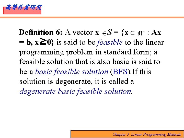
高等作業研究 Definition 6: A vector x S = {x : Ax = b, x≧ 0} is said to be feasible to the linear programming problem in standard form; a feasible solution that is also basic is said to be a basic feasible solution (BFS). If this solution is degenerate, it is called a degenerate basic feasible solution. Chapter 3 Linear Programming Methods

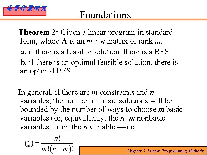
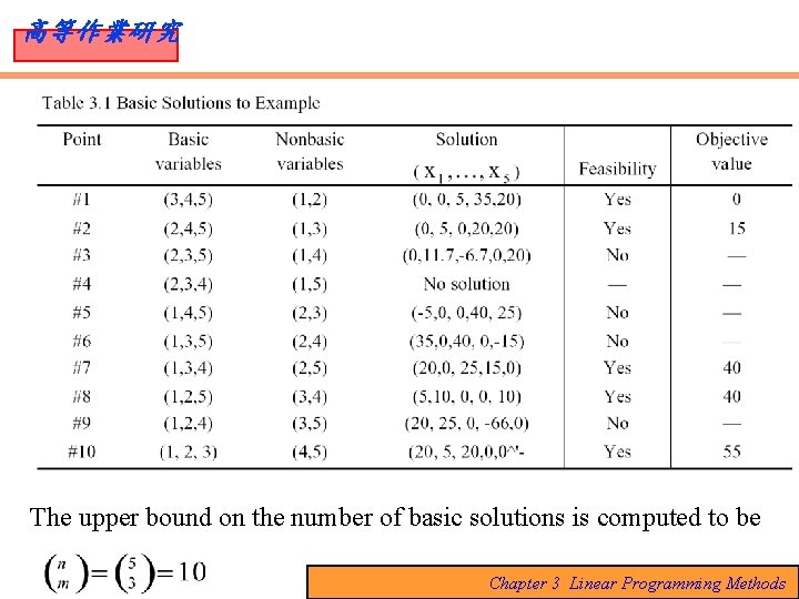
高等作業研究 Foundations Theorem 2: Given a linear program in standard form, where A is an m × n matrix of rank m, a. if there is a feasible solution, there is a BFS b. if there is an optimal feasible solution, there is an optimal BFS. In general, if there are m constraints and n variables, the number of basic solutions will be bounded by the number of ways to choose m basic variables (or, equivalently, the n -m nonbasic variables) from the n variables—i. e. , Chapter 3 Linear Programming Methods

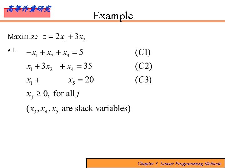
高等作業研究 Example Maximize s. t. Chapter 3 Linear Programming Methods

高等作業研究 Chapter 3 Linear Programming Methods

高等作業研究 The upper bound on the number of basic solutions is computed to be Chapter 3 Linear Programming Methods

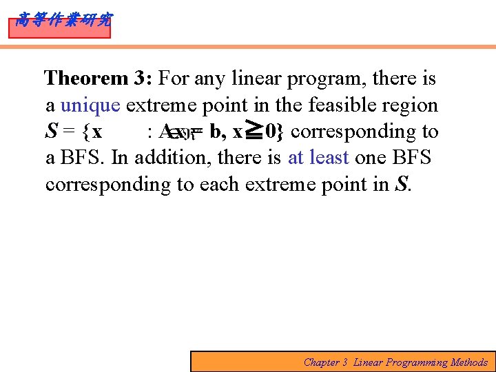
高等作業研究 Theorem 3: For any linear program, there is a unique extreme point in the feasible region S = {x : Ax = b, x≧ 0} corresponding to a BFS. In addition, there is at least one BFS corresponding to each extreme point in S. Chapter 3 Linear Programming Methods

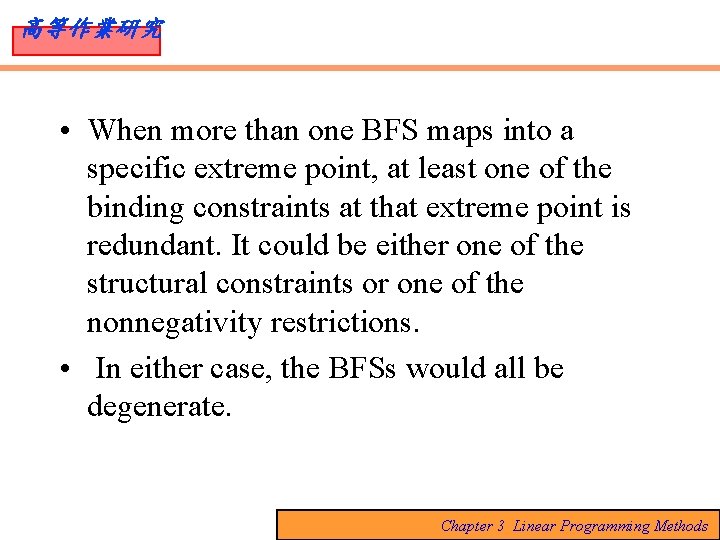
高等作業研究 • When more than one BFS maps into a specific extreme point, at least one of the binding constraints at that extreme point is redundant. It could be either one of the structural constraints or one of the nonnegativity restrictions. • In either case, the BFSs would all be degenerate. Chapter 3 Linear Programming Methods

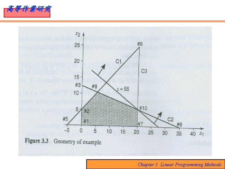
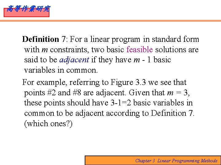
高等作業研究 Definition 7: For a linear program in standard form with m constraints, two basic feasible solutions are said to be adjacent if they have m - 1 basic variables in common. For example, referring to Figure 3. 3 we see that points #2 and #8 are adjacent. Given that m = 3, these points should have 3 -1=2 basic variables in common to be adjacent according to Definition 7. (which ones? ) Chapter 3 Linear Programming Methods

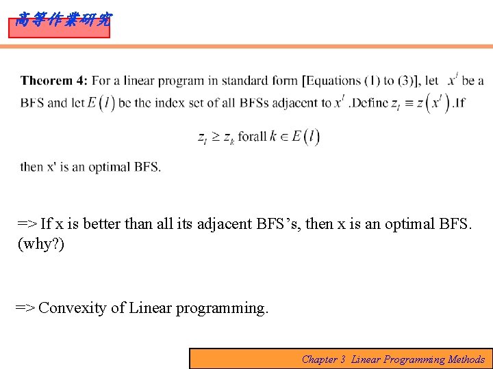
高等作業研究 => If x is better than all its adjacent BFS’s, then x is an optimal BFS. (why? ) => Convexity of Linear programming. Chapter 3 Linear Programming Methods

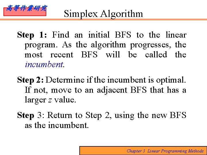
高等作業研究 Simplex Algorithm Step 1: Find an initial BFS to the linear program. As the algorithm progresses, the most recent BFS will be called the incumbent. Step 2: Determine if the incumbent is optimal. If not, move to an adjacent BFS that has a larger z value. Step 3: Return to Step 2, using the new BFS as the incumbent. Chapter 3 Linear Programming Methods

高等作業研究 • Although the number of BFSs could be huge, the simplex algorithm is seen in practice to be highly efficient. Vanderbei [1996] has empirically demonstrated that in the absence of degeneracy, approximately 0. 5(m + n) BFSs have to be examined before optimality is confirmed (when degeneracy is present, this number doubles) Chapter 3 Linear Programming Methods

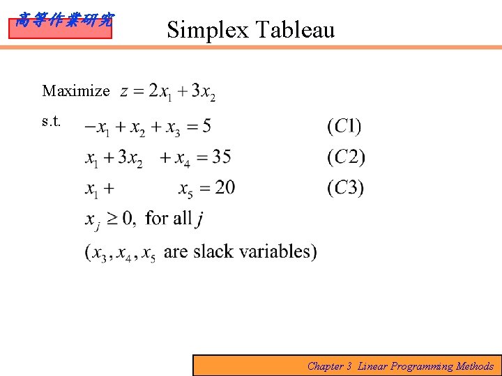
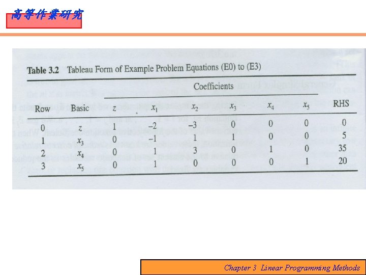
高等作業研究 Simplex Tableau Maximize s. t. Chapter 3 Linear Programming Methods

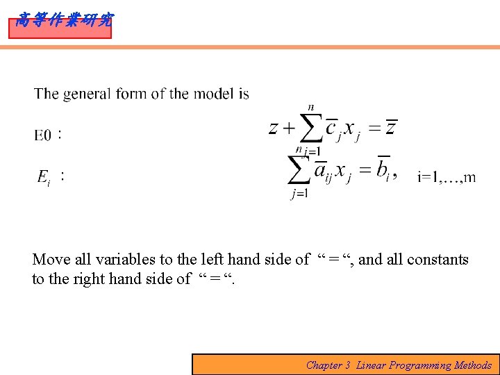
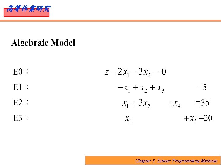
高等作業研究 Move all variables to the left hand side of “ = “, and all constants to the right hand side of “ = “. Chapter 3 Linear Programming Methods

高等作業研究 Chapter 3 Linear Programming Methods

高等作業研究 Chapter 3 Linear Programming Methods

高等作業研究 Chapter 3 Linear Programming Methods

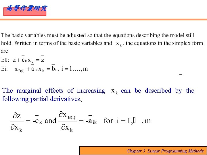
高等作業研究 The marginal effects of increasing following partial derivatives, can be described by the Chapter 3 Linear Programming Methods

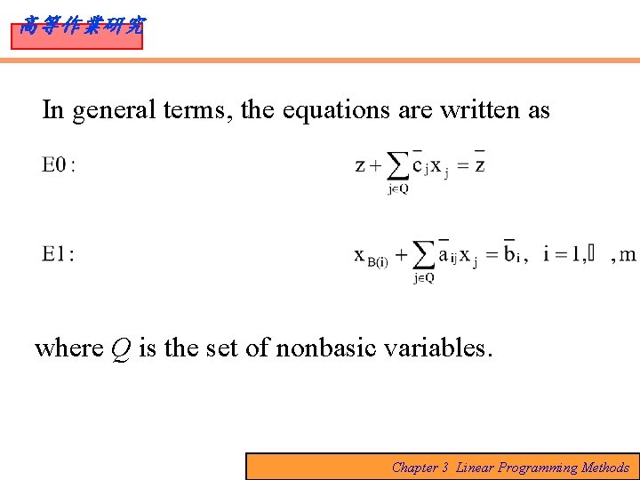
高等作業研究 In general terms, the equations are written as where Q is the set of nonbasic variables. Chapter 3 Linear Programming Methods

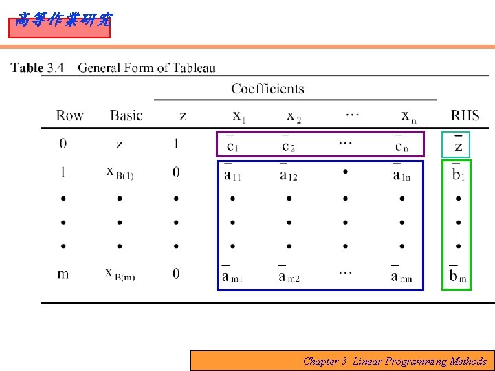
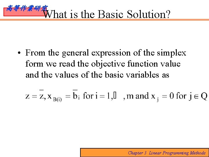
高等作業研究 What is the Basic Solution? • From the general expression of the simplex form we read the objective function value and the values of the basic variables as Chapter 3 Linear Programming Methods

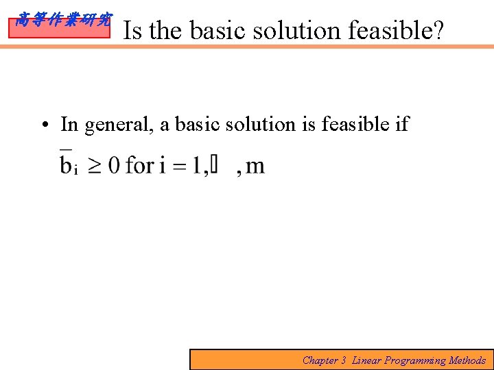
高等作業研究 Is the basic solution feasible? • In general, a basic solution is feasible if Chapter 3 Linear Programming Methods

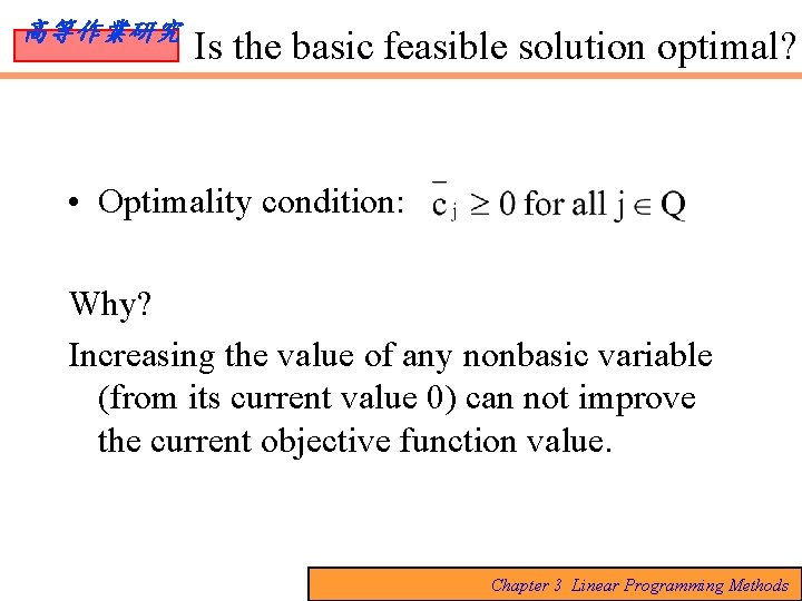
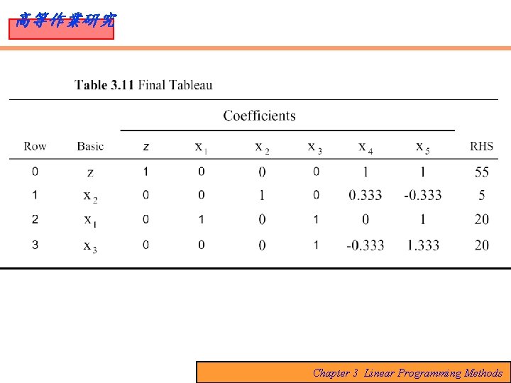
高等作業研究 Is the basic feasible solution optimal? • Optimality condition: Why? Increasing the value of any nonbasic variable (from its current value 0) can not improve the current objective function value. Chapter 3 Linear Programming Methods

高等作業研究 How Can a Nonoptimal Feasible Solution Be Improved? • The current solution can be improved by increasing any nonbasic variable with a negative coefficient in Equation E 0. • In the general case, all nonbasic variables with < 0 are candidates for conversion to basic variables. Chapter 3 Linear Programming Methods

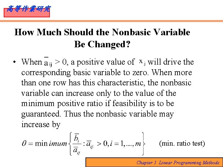
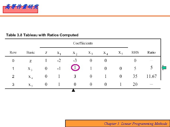
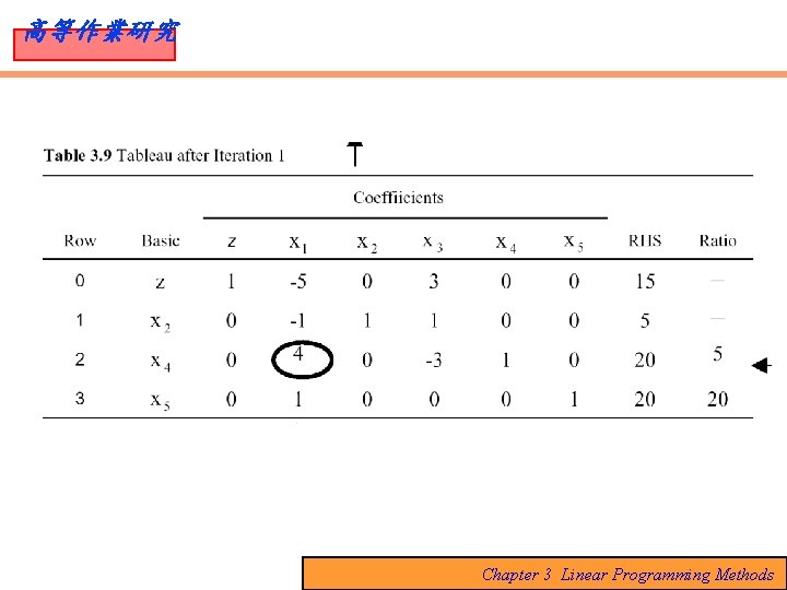
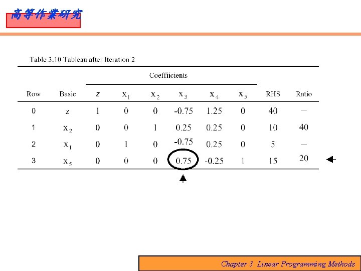
高等作業研究 How Much Should the Nonbasic Variable Be Changed? • When > 0, a positive value of will drive the corresponding basic variable to zero. When more than one row has this characteristic, the nonbasic variable can increase only to the value of the minimum positive ratio if feasibility is to be guaranteed. Thus the nonbasic variable may increase by (min. ratio test) Chapter 3 Linear Programming Methods

高等作業研究 Chapter 3 Linear Programming Methods

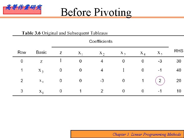
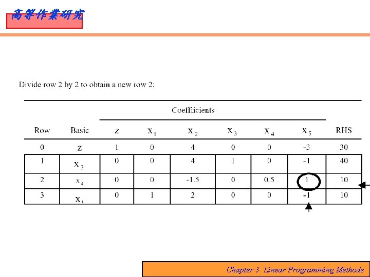
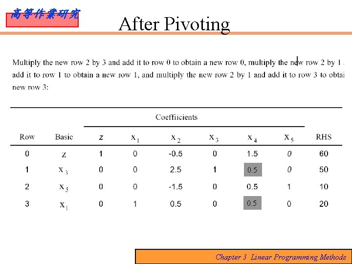
高等作業研究 How Is a New Simplex Form Obtained? The process of obtaining the new tableau is called pivoting or pricing out the entering column. It is simply a series of linear operations on the equations that results in the simplex form of the new set of basic variables. Chapter 3 Linear Programming Methods

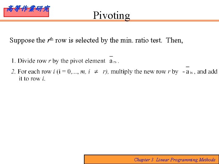
高等作業研究 Pivoting Suppose the rth row is selected by the min. ratio test. Then, Chapter 3 Linear Programming Methods

高等作業研究 Before Pivoting Chapter 3 Linear Programming Methods

高等作業研究 Chapter 3 Linear Programming Methods

高等作業研究 After Pivoting 0. 5 Chapter 3 Linear Programming Methods

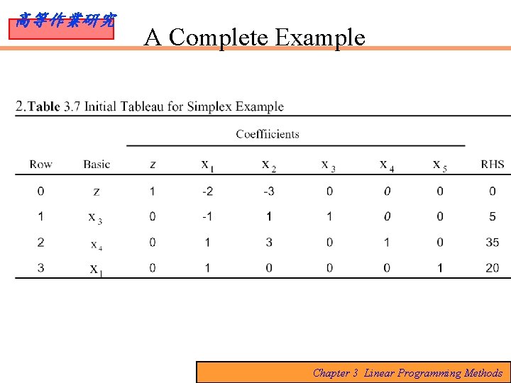
高等作業研究 A Complete Example Chapter 3 Linear Programming Methods

高等作業研究 3 Chapter 3 Linear Programming Methods

高等作業研究 Chapter 3 Linear Programming Methods

高等作業研究 Chapter 3 Linear Programming Methods

高等作業研究 Chapter 3 Linear Programming Methods

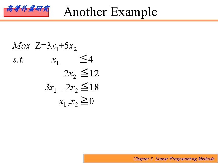
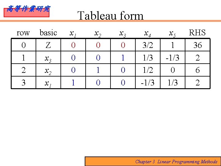
高等作業研究 Another Example Max Z=3 x 1+5 x 2 s. t. x 1 ≦ 4 2 x 2 ≦ 12 3 x 1 + 2 x 2 ≦ 18 x 1 , x 2 ≧ 0 Chapter 3 Linear Programming Methods

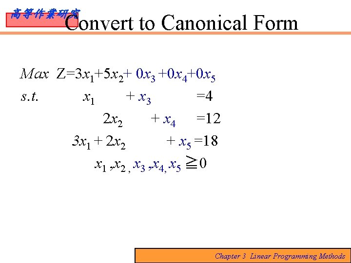
高等作業研究 Convert to Canonical Form Max Z=3 x 1+5 x 2+ 0 x 3 +0 x 4+0 x 5 s. t. x 1 + x 3 =4 2 x 2 + x 4 =12 3 x 1 + 2 x 2 + x 5 =18 x 1 , x 2 , x 3 , x 4, x 5 ≧ 0 Chapter 3 Linear Programming Methods

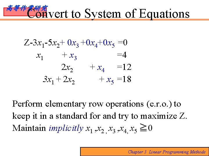
高等作業研究 Convert to System of Equations Z-3 x 1 -5 x 2+ 0 x 3 +0 x 4+0 x 5 =0 x 1 + x 3 =4 2 x 2 + x 4 =12 3 x 1 + 2 x 2 + x 5 =18 Perform elementary row operations (e. r. o. ) to keep it in a standard for and try to maximize Z. Maintain implicitly x 1 , x 2 , x 3 , x 4, x 5 ≧ 0 Chapter 3 Linear Programming Methods

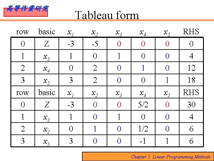
高等作業研究 row 0 1 2 3 basic Z x 3 x 4 x 5 basic Z x 3 x 2 x 5 Tableau form x 1 -3 1 0 3 x 2 -5 0 2 2 x 2 0 0 1 0 x 3 0 1 0 0 x 4 0 0 1 0 x 4 5/2 0 1/2 -1 x 5 0 0 0 1 RHS 0 4 12 18 RHS 30 4 6 6 Chapter 3 Linear Programming Methods

高等作業研究 row 0 1 2 3 basic Z x 3 x 2 x 1 Tableau form x 1 0 0 0 1 x 2 0 0 1 0 x 3 0 1 0 0 x 4 3/2 1/3 1/2 -1/3 x 5 1 -1/3 0 1/3 RHS 36 2 Chapter 3 Linear Programming Methods

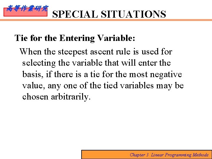
高等作業研究 SPECIAL SITUATIONS Tie for the Entering Variable: When the steepest ascent rule is used for selecting the variable that will enter the basis, if there is a tie for the most negative value, any one of the tied variables may be chosen arbitrarily. Chapter 3 Linear Programming Methods

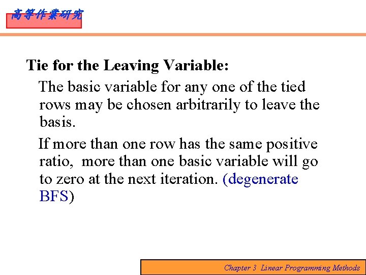
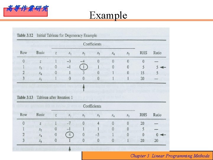
高等作業研究 Tie for the Leaving Variable: The basic variable for any one of the tied rows may be chosen arbitrarily to leave the basis. If more than one row has the same positive ratio, more than one basic variable will go to zero at the next iteration. (degenerate BFS) Chapter 3 Linear Programming Methods

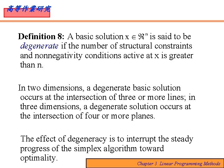
高等作業研究 Definition 8: A basic solution is said to be degenerate if the number of structural constraints and nonnegativity conditions active at x is greater than n. In two dimensions, a degenerate basic solution occurs at the intersection of three or more lines; in three dimensions, a degenerate solution occurs at the intersection of four or more planes. The effect of degeneracy is to interrupt the steady progress of the simplex algorithm toward optimality. Chapter 3 Linear Programming Methods

高等作業研究 Example Chapter 3 Linear Programming Methods

高等作業研究 • When degeneracy occurs, the possibility arises that the simplex algorithm will return to a previously encountered basis. (Cycling) • Nevertheless, cycling can be eliminated by modifying the rules used to select the entering and leaving variables. Chapter 3 Linear Programming Methods

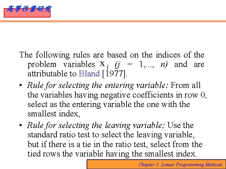
高等作業研究 The following rules are based on the indices of the problem variables (j = 1, . . . , n) and are attributable to Bland [1977]. • Rule for selecting the entering variable: From all the variables having negative coefficients in row 0, select as the entering variable the one with the smallest index, • Rule for selecting the leaving variable: Use the standard ratio test to select the leaving variable, but if there is a tie in the ratio test, select from the tied rows the variable having the smallest index. Chapter 3 Linear Programming Methods

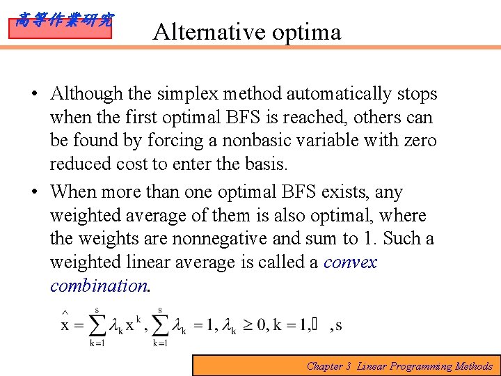
高等作業研究 Alternative optima • Although the simplex method automatically stops when the first optimal BFS is reached, others can be found by forcing a nonbasic variable with zero reduced cost to enter the basis. • When more than one optimal BFS exists, any weighted average of them is also optimal, where the weights are nonnegative and sum to 1. Such a weighted linear average is called a convex combination. Chapter 3 Linear Programming Methods

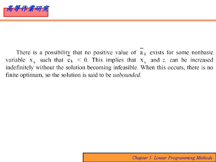
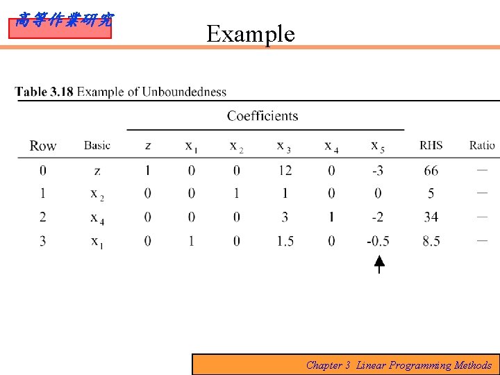
高等作業研究 Unbounded Solution • When there is a nonbasic variable with a negative coefficient in row 0 and all the other coefficients in that column are nonpositive, the value of that variable can be increased indefinitely without driving any basic variable to zero. The objective function can then be made arbitrarily large. This condition signals an unbounded solution, and there is no optimal solution for the model. The algorithm must stop if such an event occurs. Chapter 3 Linear Programming Methods

高等作業研究 Example Chapter 3 Linear Programming Methods