Chapter 3 Lecture 4 Forecasting Time Series Forecasts

Chapter 3 Lecture 4 Forecasting

Time Series Forecasts Time Series is a sequence of measurements over time, usually obtained at equally spaced intervals – Daily – Monthly – Quarterly – Yearly

Time Series Forecasts Time ordered sequence of observations taken at regular intervals. Statistical techniques that make use of historical data collected over a long period of time. Methods assume that what has occurred in the past will continue to occur in the future. Forecasts based on only one factor - time.

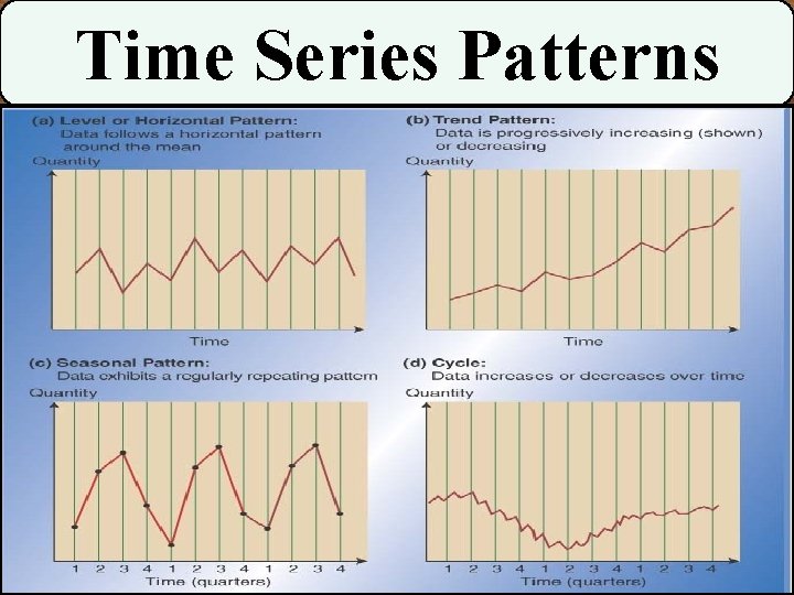
Time Series Patterns

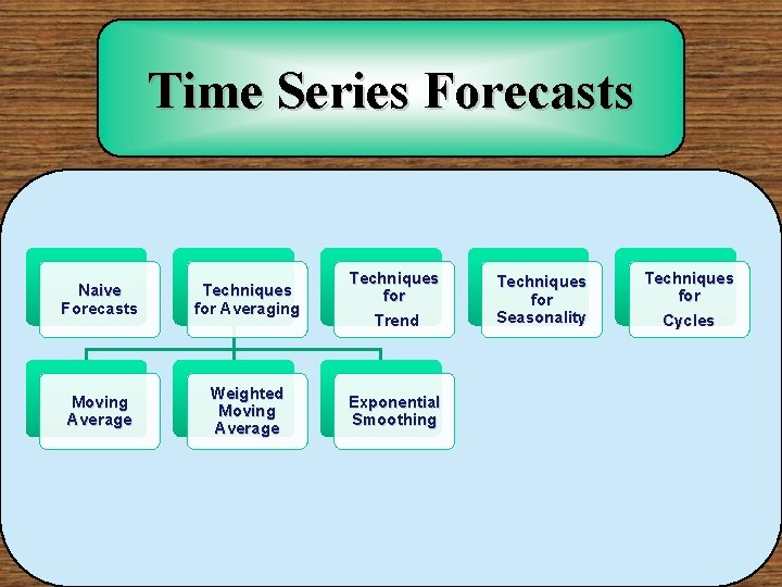
Time Series Forecasts Naive Forecasts Techniques for Averaging Techniques for Trend Moving Average Weighted Moving Average Exponential Smoothing Techniques for Seasonality Techniques for Cycles

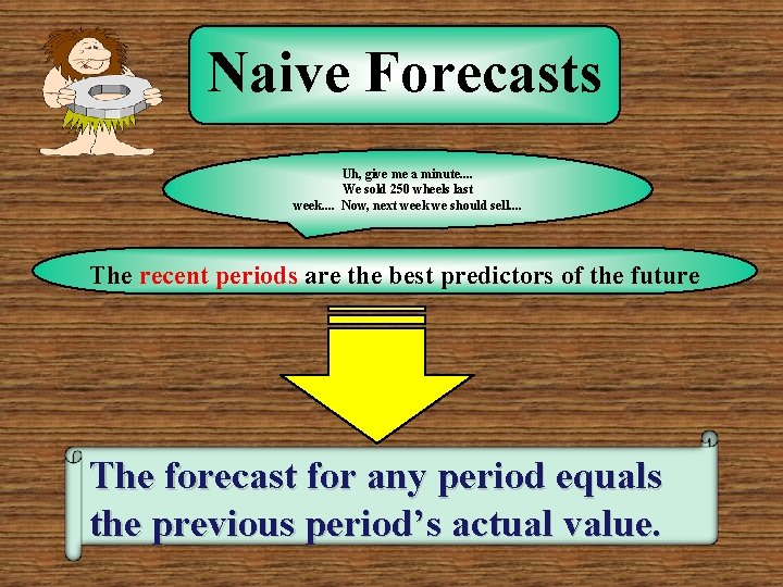
Naive Forecasts Uh, give me a minute. . We sold 250 wheels last week. . Now, next week we should sell. . The recent periods are the best predictors of the future The forecast for any period equals the previous period’s actual value.

Naïve Forecasts Simple to use Virtually no cost Quick and easy to prepare Data analysis is nonexistent Easily understandable Cannot provide high accuracy

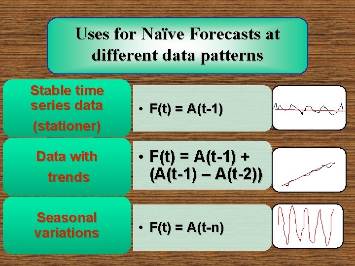
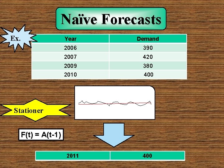
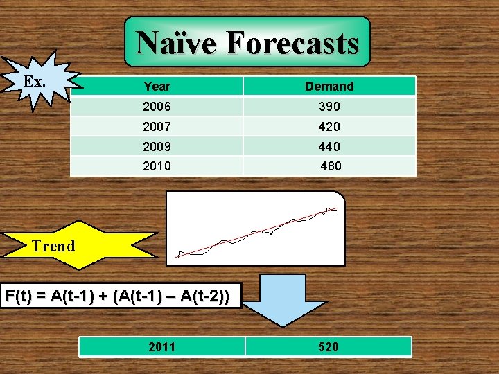
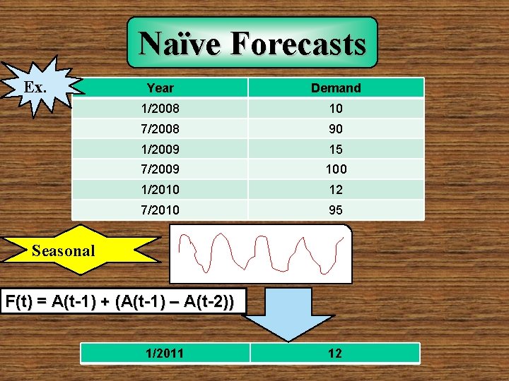
Uses for Naïve Forecasts at different data patterns Stable time series data (stationer) • F(t) = A(t-1) Data with trends • F(t) = A(t-1) + (A(t-1) – A(t-2)) Seasonal variations • F(t) = A(t-n)

Naïve Forecasts Ex. Year Demand 2006 390 2007 420 2009 380 2010 400 Stationer F(t) = A(t-1) 2011 400

Naïve Forecasts Ex. Year Demand 2006 390 2007 420 2009 440 2010 480 Trend F(t) = A(t-1) + (A(t-1) – A(t-2)) 2011 520

Naïve Forecasts Ex. Year Demand 1/2008 10 7/2008 90 1/2009 15 7/2009 100 1/2010 12 7/2010 95 Seasonal F(t) = A(t-1) + (A(t-1) – A(t-2)) 1/2011 12

Naïve Forecast Graph

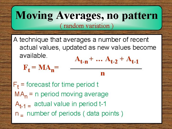
Moving Averages, no pattern ( random variation ) A technique that averages a number of recent actual values, updated as new values become available. Ft = MAn= At-n + … At-2 + At-1 n Ft = forecast for time period t MAn = n period moving average At-1 = actual value in period t-1 n = number of periods ( data points )

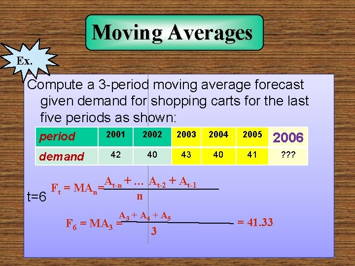
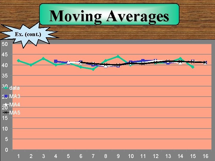
Moving Averages Ex. Compute a 3 -period moving average forecast given demand for shopping carts for the last five periods as shown: 2001 2002 2003 2004 2005 period 2006 demand 42 40 43 40 41 At-n + … At-2 + At-1 Ft = MAn= n t=6 A 3 + A 4 + A 5 F 6 = MA 3 = 41. 33 ? ? ?

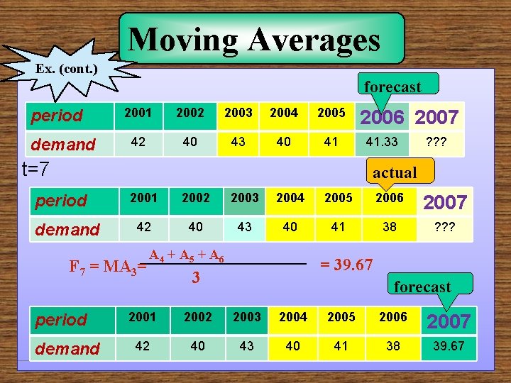
Moving Averages Ex. (cont. ) forecast period demand 2001 2002 2003 2004 2005 42 40 43 40 41 2006 2007 41. 33 t=7 ? ? ? actual period demand 2001 2002 2003 2004 2005 2006 2007 42 40 43 40 41 38 ? ? ? F 7 = MA 3= period demand A 4 + A 5 + A 6 = 39. 67 3 forecast 2001 2002 2003 2004 2005 2006 2007 42 40 43 40 41 38 39. 67

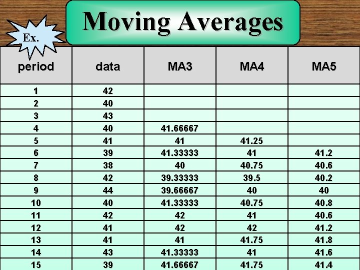
Ex. Moving Averages period data MA 3 MA 4 MA 5 1 2 3 4 5 6 7 8 9 10 11 12 13 14 15 42 40 43 40 41 39 38 42 44 40 42 41 41 43 39 41. 66667 41 41. 33333 40 39. 33333 39. 66667 41. 33333 42 42 41 41. 33333 41. 66667 41. 25 41 40. 75 39. 5 40 40. 75 41 42 41. 75 41. 2 40. 6 40. 2 40 40. 8 40. 6 41. 2 41. 8 41. 6 41. 4

Moving Averages Ex. (cont. ) 50 45 40 35 30 data 25 MA 3 MA 4 20 MA 5 15 10 5 0 1 2 3 4 5 6 7 8 9 10 11 12 13 14 15 16

Ex. Moving Averages

Moving Averages Ex. (cont. )

Ex. Moving Averages

Stability vs. Responsiveness • Should I use a 2 -period moving average or a 3 period moving average? • The larger the “n” the more stable the forecast. • A 2 -period model will be more responsive to change. • We must balance stability with responsiveness • If responsiveness is required, average with few data points should be used,

Moving Averages Decreasing the number of data points in an moving average technique, increase the weight of more recent values As data points in an moving average technique increased, the sensitivity ( responsiveness ) of the average to new values decreased. If responsiveness is required, average with few data points should be used,

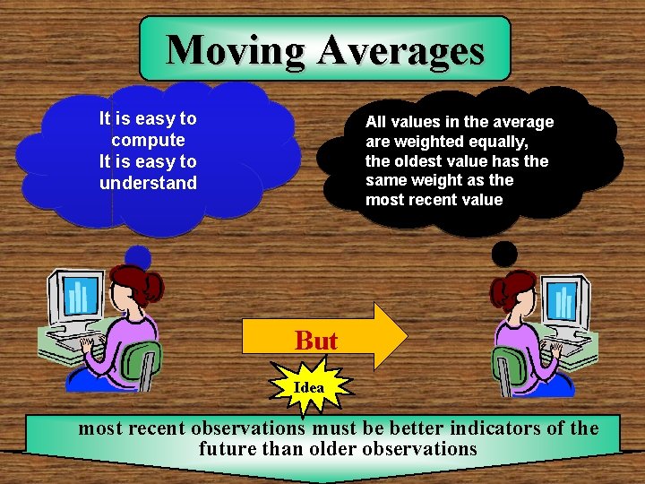
Moving Averages It is easy to compute It is easy to understand All values in the average are weighted equally, the oldest value has the same weight as the most recent value But Idea most recent observations must be better indicators of the future than older observations

Weighted Moving Averages Historical values of the time series are assigned different weights when performing the

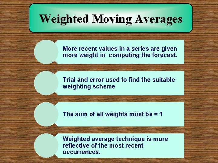
Weighted Moving Averages More recent values in a series are given more weight in computing the forecast. Trial and error used to find the suitable weighting scheme The sum of all weights must be = 1 Weighted average technique is more reflective of the most recent occurrences.

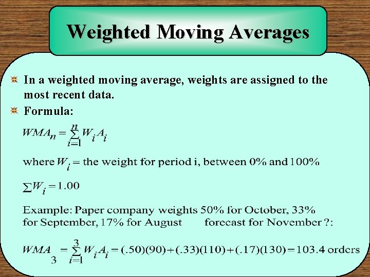
Weighted Moving Averages In a weighted moving average, weights are assigned to the most recent data. Formula:

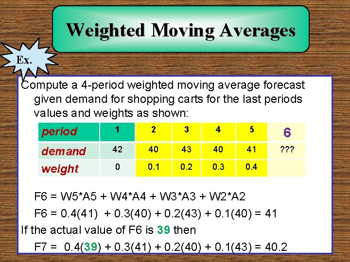
Weighted Moving Averages Ex. Compute a 4 -period weighted moving average forecast given demand for shopping carts for the last periods values and weights as shown: period 1 2 3 4 5 6 demand weight 42 40 43 40 41 ? ? ? 0 0. 1 0. 2 0. 3 0. 4 F 6 = W 5*A 5 + W 4*A 4 + W 3*A 3 + W 2*A 2 F 6 = 0. 4(41) + 0. 3(40) + 0. 2(43) + 0. 1(40) = 41 If the actual value of F 6 is 39 then F 7 = 0. 4(39) + 0. 3(41) + 0. 2(40) + 0. 1(43) = 40. 2

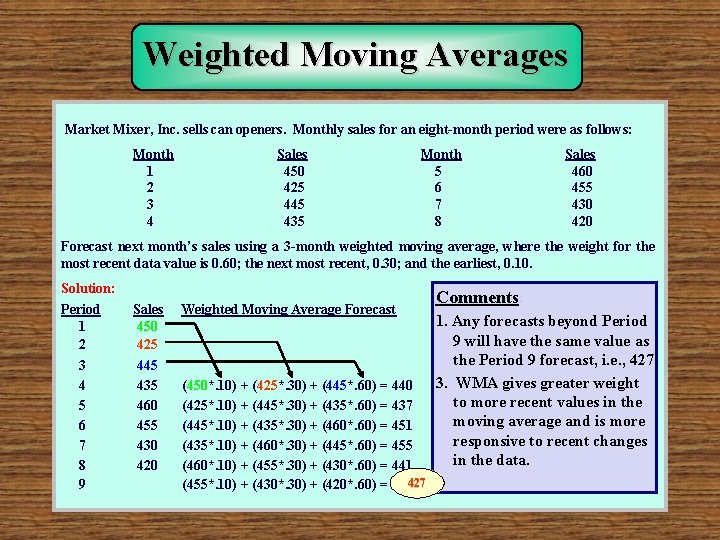
Weighted Moving Averages Market Mixer, Inc. sells can openers. Monthly sales for an eight-month period were as follows: Month 1 2 3 4 Sales 450 425 445 435 Month 5 6 7 8 Sales 460 455 430 420 Forecast next month’s sales using a 3 -month weighted moving average, where the weight for the most recent data value is 0. 60; the next most recent, 0. 30; and the earliest, 0. 10. Solution: Period 1 2 3 4 5 6 7 8 9 Sales 450 425 445 435 460 455 430 420 Weighted Moving Average Forecast (450*. 10) + (425*. 30) + (445*. 60) = 440 (425*. 10) + (445*. 30) + (435*. 60) = 437 (445*. 10) + (435*. 30) + (460*. 60) = 451 (435*. 10) + (460*. 30) + (445*. 60) = 455 (460*. 10) + (455*. 30) + (430*. 60) = 441 (455*. 10) + (430*. 30) + (420*. 60) = 427 Comments: 1. Any forecasts beyond Period 9 will have the same value as the Period 9 forecast, i. e. , 427. 3. WMA gives greater weight to more recent values in the moving average and is more responsive to recent changes in the data.

Exponential Smoothing • The most recent observations might have the highest predictive value. • Therefore, we should give more weight to the more recent time periods when forecasting.

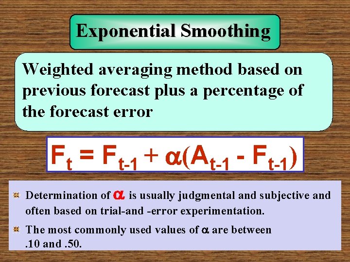
Exponential Smoothing Weighted averaging method based on previous forecast plus a percentage of the forecast error Ft = Ft-1 + (At-1 - Ft-1) Determination of is usually judgmental and subjective and often based on trial-and -error experimentation. The most commonly used values of are between. 10 and. 50.

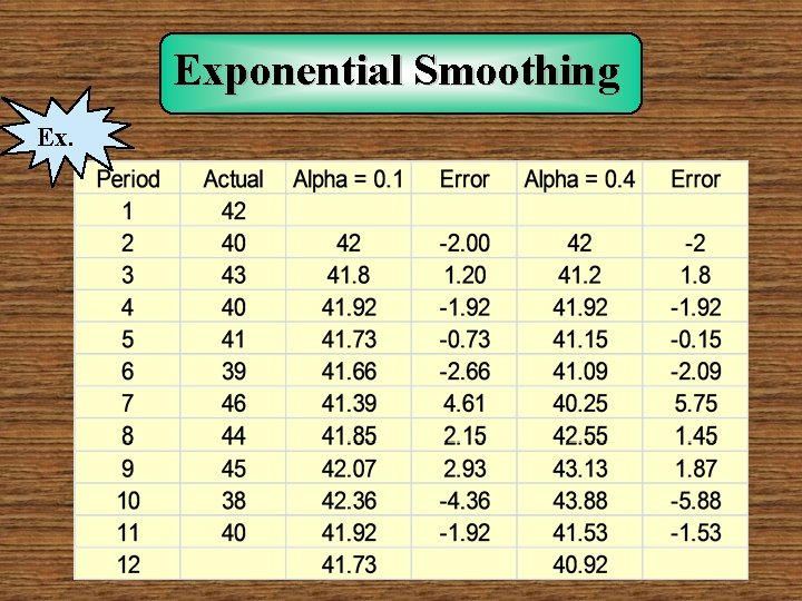
Exponential Smoothing Ex.

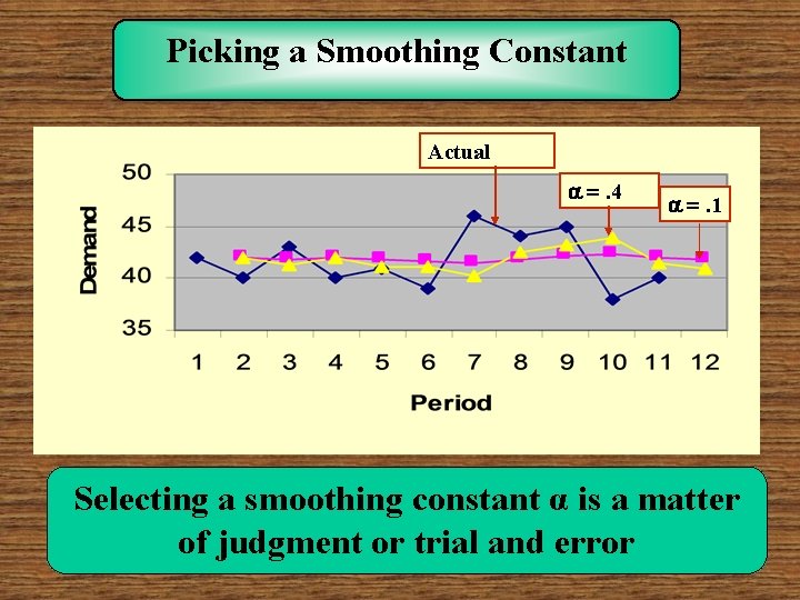
Picking a Smoothing Constant Actual . 4 . 1 Selecting a smoothing constant α is a matter of judgment or trial and error

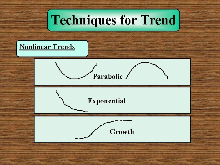
Techniques for Trend Nonlinear Trends Parabolic Exponential Growth

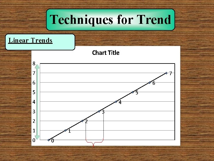
Techniques for Trend Linear Trends

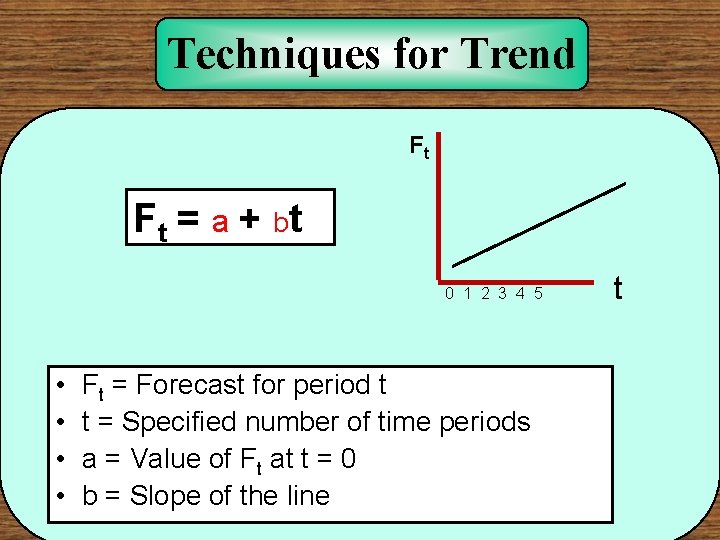
Techniques for Trend Ft F t = a + bt 0 1 2 3 4 5 • • Ft = Forecast for period t t = Specified number of time periods a = Value of Ft at t = 0 b = Slope of the line t

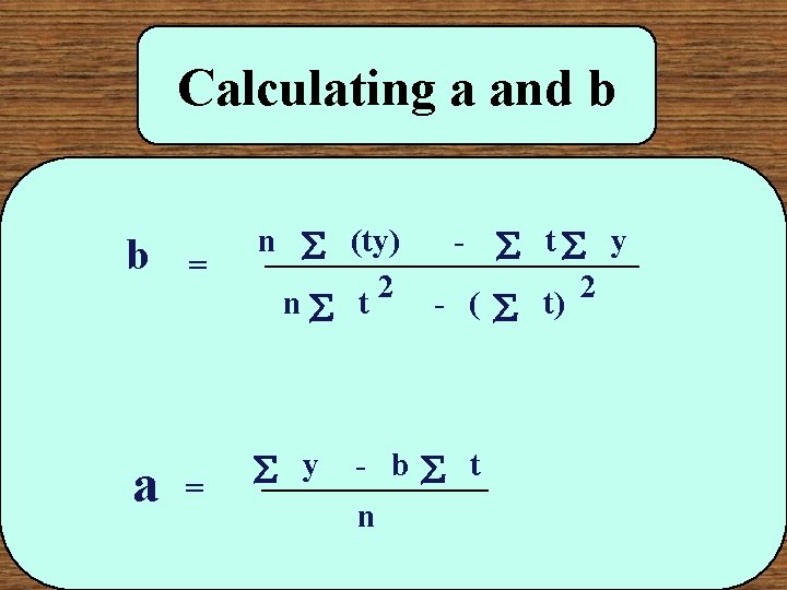
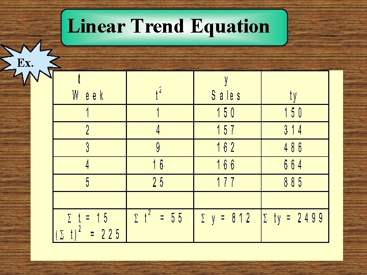
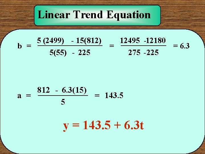
Calculating a and b b a = = n (ty) 2 n t y t y 2 - ( t) - - b t n

Linear Trend Equation Ex.

Linear Trend Equation 5 (2499) - 15(812) b = 5(55) - 225 12495 -12180 = = 6. 3 275 -225 812 - 6. 3(15) a = = 143. 5 5 y = 143. 5 + 6. 3 t

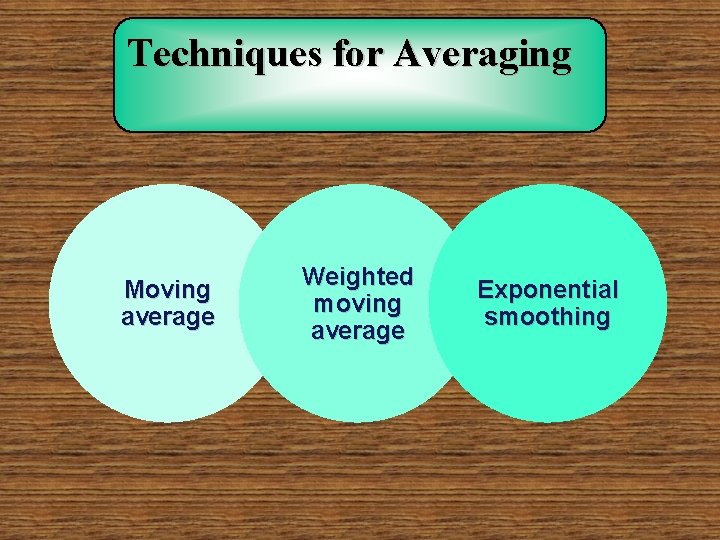
Techniques for Averaging Moving average Weighted moving average Exponential smoothing