CHAPTER 3 Key Principles of Statistical Inference Objectives

CHAPTER 3 Key Principles of Statistical Inference

Objectives for Chapter 3 o Describe the principles of statistical inference o Describe characteristics of a normal distribution o Discuss types of hypothesis-testing o Discuss Type 1 & Type II statistical errors

Objectives for Chapter 3 o Define sensitivity, specificity, predictive value & efficiency o Discuss tests of significance o Interpret a confidence interval o Examine the components of sample size estimation for study populations

Statistical Inference o Involves obtaining information from sample of data about population from which sample was drawn & setting up a model to describe this population o When random sample is drawn from population, every member of population has equal chance of being selected in the sample

Finite Population o Each person in population can be listed o Random sample can be drawn using: n n n Table of random numbers Research Randomizer http: //www. randomizer. org Random. Org http: //www. random. org

Types of Statistical Inference o Parameter Estimation takes two forms n Point Estimation: when estimate of population parameter is single number p Ex. Mean, median, variance & SD o Hypothesis-Testing: n More common type

Normal Curve o Theoretically perfect frequency polygon in which mean, median & mode all coincide in center o Takes form of symmetrical bell-shaped curve o Called Gaussian Curve o Most important distribution in statistics
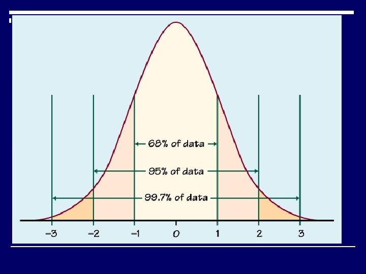

Normal Curve • 68% of cases fall within + 1 SD of the mean • 95% of cases fall within + 2 SD of the mean • 99. 7% of cases fall within + 3 SD of the mean.

Normal Distribution & Z score o When variable’s mean & SD are known, any set of scores can be transformed into zscores with n Mean = 0 SD = 1 o Two Important Z scores: n n + 1. 96 z = 95% confidence interval + 2. 58 z = 99% confidence interval

USEFULNESS OF Z-SCORES o Can make comparisons across different normal distributions, across different samples of individuals or different groups. o The Z score standardizes all normal curves, makes them comparable even when the means and standard deviations are different.

Percentiles o Tells the relative position of a given score o Allows us to compare scores on tests with different means & SDs. o Calculated as o (# of scores - given score) X 100 total # of scores

Percentile o 25 th percentile = 1 st quartile o 50 th percentile = 2 nd quartile Also the median o 75 th percentile = 3 rd quartile

Standard Scores o Way of expressing a score in terms of its relative distance from the mean n z-score is example of standard score o Standard scores are used more often than percentiles o Transformed standard scores often called T-scores n Usually has M = 50 & SD = 10

Normal Distribution & Drawing Samples o When many samples are drawn from a population, the means of those samples tend to be normally distributed o Larger the number of samples, the more the distribution approximates the normal curve
 o Is standard deviation of the population o Constant")
Standard Error of Mean (SE) o Is standard deviation of the population o Constant relationship between SD of a distribution of sample means (SE), the SD of population from which samples were drawn & size of samples o As size of sample increases, size of error decreases o The greater the variability, the greater the error

Probability Axioms o Fall between 0% & 100% o No negative probabilities o Probability of an event is 100% less the probability of the opposite event

Definitions of Probability o Frequency Probability based on number of times an event occurred in a given sample (n) # of times event occurred X 100 total # of people in n

Definitions of Probability o Subjective Probability: percentage expressing personal, subjective belief that event will occur o p values of. 05, often used as a probability cutoff in hypothesis-testing to indicate something unusual happening in the distribution

Hypothesis-Testing o Prominent feature of quantitative research o Hypotheses originate from theory that underpins research o Two types of hypotheses: n n Null Ho Alternative

Null Hypothesis - Ho o Ho proposes no difference or relationship exists between the variables of interest o Foundation of the statistical test o When you statistically test an hypothesis, you assume that Ho correctly describes the state of affairs between the variables of interest

Null Hypothesis - Ho o If a statistically significant relationship is found (p <. 05), Ho is rejected o If no statistically significant relationship is found (p. >. 05), Ho is rejected

Alternative Hypothesis - Ha o A hypothesis that contradicts Ho o Can indicate the direction of the difference or relationship expected o Often called the research hypothesis & represented by Hr

Sampling Error o Inferences from samples to populations are always probabilistic, meaning we can never be certain our inference was correct o Drawing the wrong conclusion is called an error of inference, defined in terms of Ho as Type I and Type II

Types of Errors o We summarize these in a 2 x 2 box: H 0 True H 0 False Reject H 0 Right decision Wrong decision 1 -b Retain H 0 Wrong decision 1 - Right decision b

Types of Errors o Type I error occurs when you reject a true Ho n Called alpha error o Type II error occurs when you accept a false Ho n Called beta error

Types of Errors o Inverse relationship between Type 1 & Type II errors. n n Decreasing the likelihood of one type of error increases the likelihood of the other type error This can be done by changing the significance level o Which type of error can be most tolerated in a particular study?

Screening for Diseases o. Sensitivity o. Specificity o. Predictive Value o. Efficiency

Why Screen? o Tenet of public health is that primary prevention is best o If all cases of disease cannot be prevented, then the next best strategy is the early detection of disease in asymptomatic, apparently healthy individuals

Questions to Ask o Based on disease status: n If we screen a population, what proportion of people who have the disease will be correctly identified? n If we screen a population, what proportion of people who do not have the disease will be correctly identified?

Questions to Ask o Based on the test results: n If the test result is positive, what is the probability that the patient will have the disease? n If the test result is negative, what is the probability that the patient will not have the disease?

Sensitivity & Specificity o Sensitivity: The ability of a test to correctly identify those with the disease (true positives) o Specificity: The ability of a test to correctly identify those without the disease (true negatives)

Ideal Screening Test o 100% sensitive = No false negatives o 100% specific = No false positives
 POSITIVE (+) Actual diagnosis Not Diseased")
An Ideal Screening Program… TEST RESULTS NEGATIVE (-) POSITIVE (+) Actual diagnosis Not Diseased True Negative (TN) CORRECT Diseased True Positive (TP) CORRECT
 POSITIVE (+) Actual diagnosis Not Diseased")
In the real world… TEST RESULTS NEGATIVE (-) POSITIVE (+) Actual diagnosis Not Diseased True Negative (TN) False Negative (FN) False Positive (FP) True Positive (TP) CORRECT Oops! Should not have these CORRECT
 test result.")
More Definitions o False Positive: Healthy person incorrectly receives a positive (diseased) test result. o False Negative: Diseased person incorrectly receives a negative (healthy) test result.

2 x 2 Table to Calculate Various Outcomes True Diagnosis Diseased a Positive Test Result TP c Negative Total Not Diseased b FP a+b TN c+d d FN a+c Total b+d a+b+c+d
 Diseased a TP Positive Test Result c b")
Calculating Sensitivity True Diagnosis Sensitivity (Sn) Diseased a TP Positive Test Result c b FN a+c Total FP a+b TN c+d d Negative Total Not Diseased b+d a+b+c+d o The probability of having a positive test if you are positive (diseased) a Sensitivity = (a + c) True Positives = True Positives + False Negatives
 Diseased a Positive Test Result TP c Total")
Calculating Specificity True Diagnosis Specificity (Sp) Diseased a Positive Test Result TP c Total b a+c Total FP a+b TN c+d d FN Negative Not Diseased b+d a+b+c+d o The probability of having a negative test if you are negative (not diseased) Specificity = True Negatives d (b + d) = False Positives + True Negatives

Inverse Relationships o o % Sensitivity + % False Negative = 100% n Higher sensitivity fewer false negatives n Lower sensitivity more false negatives % Specificity + % False Positive = 100% n Higher specificity fewer false positives n Lower specificity more false positives

Number of Individuals Interrelationship Between Sensitivity and Specificity B true negatives A C true positives Normal (no disease) false negatives Diseased false positives

Example: 80 people had their serum level of calcium checked to determine whether they had hyperparathyroidism. 20 were ultimately shown to have the disease. Of the 20, 12 had an elevated level of calcium (positive test result). Of the 60 determined to be free of disease, 3 had an elevated level of calcium. Step 1: Fill in the boxes with the data provided True Diagnosis Diseased a Positive Test Result 12 c Not Diseased b Total 3 d Negative Total 20 60 80

Example: 80 people had their serum level of calcium checked to determine whether they had hyperparathyroidism. 20 were ultimately shown to have the disease. Of the 20, 12 had an elevated level of calcium (positive test result). Of the 60 determined to be free of disease, 3 had an elevated level of calcium. Step 2: Complete the table True Diagnosis Diseased a Positive Test Result 12 c Not Diseased b Total 3 15 d Negative 8 57 65 Total 20 60 80

Step 3: Calculating the Sensitivity True Diagnosis Diseased a 12 Positive Test Result c Negative 8 Total 20 Sensitivity = a (a + c) = 12/20 = 60% Not Diseased b d Total 3 15 57 65 60 80 True Positives + False Negatives

Step 4: Calculating the Specificity True Diagnosis Diseased a 12 Positive Test Result c Negative 8 Total 20 Specificity = d (b + d) = 57/60 = 95% Not Diseased b d Total 3 15 57 65 60 80 True Negatives False Positives + True Negatives

Which is Preferred: High Sensitivity or High Specificity? o If you have a fatal disease with no treatment (such as for early cases of AIDS), optimize specificity o If you are screening to prevent transmission of a preventable disease (such as screening for HIV in blood donors), optimize sensitivity
 of false positive and false negative test results. o")
Goal o Minimize chance (probability) of false positive and false negative test results. o Or, equivalently, maximize probability of correct results.

Accuracy of tests in use o Positive predictive value: probability that a person who has a positive test result really has the disease. o Negative predictive value: probability that a person who has a negative test result really is healthy.

Example
 Positive predictive value = 49/1467 = 0. 033 Negative predictive value =")
Example (continued) Positive predictive value = 49/1467 = 0. 033 Negative predictive value = 1475/1511 = 0. 98 Kids who test positive have small chance in having elevated lead levels, while kids who test negative can be quite confident that they have normal lead levels.

Caution about predictive values! Reading positive and negative predictive values directly from table is accurate only if the proportion of diseased people in the sample is representative of the proportion of diseased people in the population. (Random sample!)

Example
 o Sn = 392/400 = 0. 98 o Sp = 576/600 =")
Example (continued) o Sn = 392/400 = 0. 98 o Sp = 576/600 = 0. 96 o PPV = 392/416 = 0. 94 o NPV = 576/584 = 0. 99 Looks good? Note prevalence of disease is 400/1000 or 40%

Example
 o Sn = 49/50 = 0. 98 o Sp = 912/950 =")
Example (continued) o Sn = 49/50 = 0. 98 o Sp = 912/950 = 0. 96 o PPV = 49/87 = 0. 56 o NPV = 912/913 = 0. 999 Sensitivity & specificity the same, but PPV smaller because prevalence of disease is smaller, namely 50/1000 or 5%.

Find correct predictive values by knowing…. o True proportion of diseased people in the population. o Sensitivity of the test o Specificity of the test

Example: PPV of pap smears? o Rate of atypia in normal population is 0. 001 o Sensitivity = 0. 70 o Specificity = 0. 90 Find probability that a woman will have atypical cervical cells given that she had a positive pap smear.

Example

Example

Example

Example

Example
 o PPV = 70/10, 060 = 0. 00696 o NPV = 89,")
Example (continued) o PPV = 70/10, 060 = 0. 00696 o NPV = 89, 910/89, 940 = 0. 999 Person with positive pap has tiny chance (0. 6%) of truly having disease, while person with negative pap almost certainly will be disease free.

Significance Level o States risk of rejecting Ho when it is true o Commonly called p value n n n Ranges from 0. 00 - 1. 00 Summarizes the evidence in the data about Ho Small p value of. 001 provides strong evidence against Ho, indicating that getting such a result might occur 1 out of 1, 000 times

Testing a Statistical Hypothesis o State Ho o Choose appropriate statistic to test Ho o Define degree of risk of incorrectly concluding Ho is false when it is true o Calculate statistic from a set of randomly selected observations o Decide whether to accept or reject Ho based on sample statistic

Power of a Test o Probability of detecting a difference or relationship if such a difference or relationship really exists o Anything that decreases the probability of a Type II error increases power & vice versa o A more powerful test is one that is likely to reject Ho

One-Tailed & Two-Tailed Tests o Tails refer to ends of normal curve o When we hypothesize the direction of the difference or relationship, we state in what tail of the distribution we expect to find the difference or relationship o One-tailed test is more powerful & is used when we have a directional hypothesis

Tailedness Significantly different from mean Tail . 025 Significantly different from mean Tail Two-Tailed Test-. 05 Level of Significance . 05 Significantly different from mean One-Tailed Test-. 05 Level of Significance
 o The freedom of a score’s value to vary given")
Degrees of Freedom (df) o The freedom of a score’s value to vary given what is known about other & the sum of the scores n n Ex. Given three scores, we have 3 df, one for each independent item. Once you know mean, we lose one df df = n - 1, the number of items in set less 1
 o Degree of confidence, expressed as a percent, that the interval")
Confidence Interval (CI) o Degree of confidence, expressed as a percent, that the interval contains the population mean (or proportion), & for which we have an estimate calculated from sample data n n 95% CI = X + 1. 96 (standard error) 99% CI = X + 2. 58 (standard error)
")
Relationship Between Confidence Interval & Significance Levels o 95% CI contains all the (Ho) values for which p >. 05 o Makes it possible to uncover inconsistencies in research reports o A value for Ho within the 95% CI should have a p value >. 05, & one outside of the 95% CI should have a p value less than. 05

Statistical Significance VS Meaningful Significance o Common mistake is to confuse statistical significance with substantive meaningfulness o Statistically significant result simply means that if Ho were true, the observed results would be very unusual o With N > 100, even tiny relationships/differences are statistically significant

Statistical Significance VS Meaningful Significance o Statistically significant results say nothing about clinical importance or meaningful significance of results o Researcher must always determine if statistically significant results are substantively meaningful. o Refrain from statistical “sanctification” of data

Sample Size Determination o Likelihood of rejecting Ho (ie, avoiding a Type II error o Depends on n Significance Level: P value, usually. 05 Power: 1 - beta error, usually set at. 80 Effect Size: degree to which Ho is false (ie, the size of the effect of independent variable on dependent variable
 can be")
Sample Size Determination o Given three of these parameters, the fourth (n) can be determined o Can use Sample Size tables to determine the optimal n needed for a given analysis
- Slides: 75