Chapter 3 isentropic analysis 3 1 3 2

Chapter 3: isentropic analysis 3. 1 3. 2 3. 3 isentropic coordinate system isentropic chart interpretation vertical motion on isentropic charts

isentropic coordinates derivation of the equations of motion in isentropic coordinates: on blackboard isobaric coordinates isentropic coordinates pros and cons of isentropic coordinates can be found in this meted module, by J. Moore

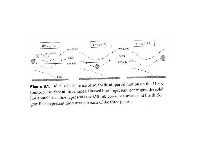
Isentropic maps: some examples infer vertical motion – low levels L 800 850 900 285 K

Isentropic maps: some examples same time, higher level 450 900 295 K

295 K – relative humidity suggests that storm-relative motion has an easterly component in E Montana

Isentropic maps: some examples same time, upper levels infer vertical motion – relate to QG argument 325 K 200 300 200 500

sample isentropic charts showing winds, pressure, and winds 280 K • College of Dupage • OU 2014/03/28/12 Z 310 K 290 K

2014/03/28/12 Z

diagnosing vertical motion on isentropic charts: impact of storm motion time 1 c time 1 time 2 (u, v)storm-relative = (u, v) - c This is discussed further in Section 6 of this meted module, by J. Moore

vertical motion & diabatic processes layer perspective parcel perspective

textbook case study: 3 Jan 2002, 00 UTC 296 K surface

500 mb height & abs vort - same time

500 mb height & SLP same time

500 mb height & Q vectors & Q divergence - same time

500 mb height & 700 mb omega - same time

x Greensboro IDV 3 D plot of 296 K isentropic surface wind vectors on this surface same time (00 Z on 3 Jan 2002)

Greensboro (GSO) sounding same time

GSO pressure and winds on the 296 K isentropic surface same time

296 K pressure & wind 296 K pressure & storm-relative wind c = 8. 5 m/s towards the ESE

296 K pressure & storm-relative wind & mixing ratio (g/kg) – same time

296 K pressure & storm-relative wind & precipitation (d. BZ) – same time