Chapter 3 Introduction to optimization models Linear Programming

Linear Programming • The PCTech company makes and sells two models for computers, Basic

Linear Programming • PC Tech wants to know how many of each model it

x 2 Graphical Method x 1 = Number of basic computer model x 2

Graphical Method x 2 1800 x 1 = Number of basic computer model x

Graphical Method x 2 1800 Net profit = 80 x 1 + 129 x

Constraints Labor hours constraints Assembly labor Testing labor Basic Model XP Model Hours available

x 2 Assembly Hours Constraints 1800 X 1 = 0, x 2 = 1666.

x 2 Testing Hours Constraints 1800 X 1 = 0, x 2 = 1500

x 2 Maximum sales Constraints 1800 x 1 = Number of basic computer model

x 2 Maximum sales Constraints 1800 X 1 = 0, x 2 = 1200

x 2 Feasible region 1800 x 1 = Number of basic computer model x

x 2 Optimum solution 1800 x 1 = Number of basic computer model x

x 2 Optimum solution 1800 Optimum solution 1600 1400 x 1 = Number of

The algebraic model Maximize 80 x 1 + 129 x 2 subject to: 5

Elements of LP model • Decision variables – The variable whose values must be

LP requirements • • • Proportionality of variables Additivity of resources Divisibility of variables

Scaling in LP • Poorly scaled model – model contains some very large numbers

Solutions to LP problem • Feasible solution • Feasible region • Optimal solution –

x 2 Multiple Optimum solution 1800 x 1 = Number of basic computer model

Unbounded Solution x 2 1800 x 1 = Number of basic computer model x

Infeasible Solution x 2 1800 x 1 = Number of basic computer model x

Summary • An LP model may result in – an unique optimum solution –

Slides: 26

Download presentation

Chapter 3 Introduction to optimization models

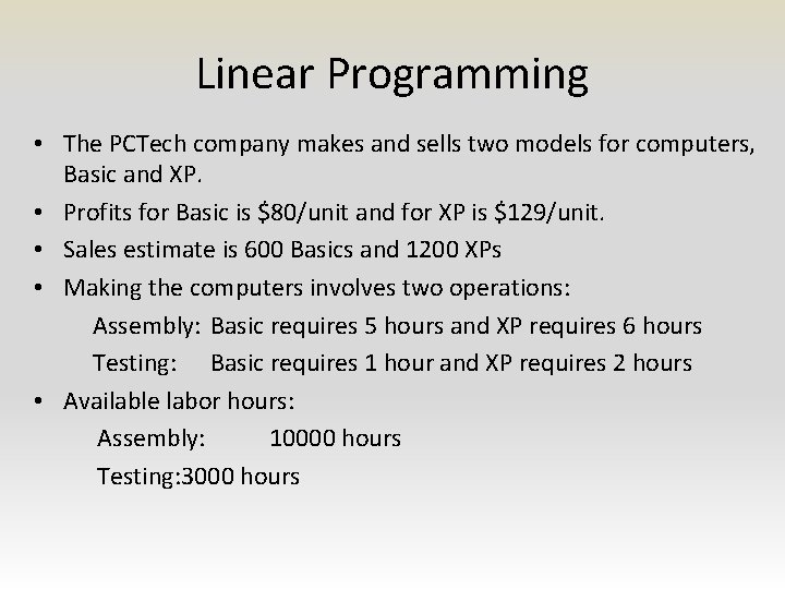
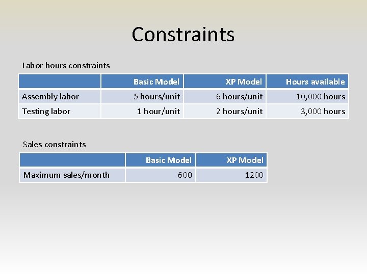
Linear Programming • The PCTech company makes and sells two models for computers, Basic and XP. • Profits for Basic is $80/unit and for XP is $129/unit. • Sales estimate is 600 Basics and 1200 XPs • Making the computers involves two operations: Assembly: Basic requires 5 hours and XP requires 6 hours Testing: Basic requires 1 hour and XP requires 2 hours • Available labor hours: Assembly: 10000 hours Testing: 3000 hours

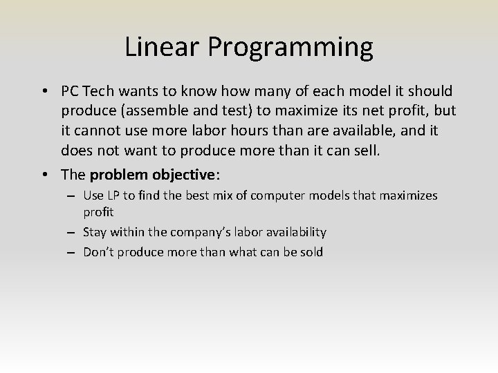
Linear Programming • PC Tech wants to know how many of each model it should produce (assemble and test) to maximize its net profit, but it cannot use more labor hours than are available, and it does not want to produce more than it can sell. • The problem objective: – Use LP to find the best mix of computer models that maximizes profit – Stay within the company’s labor availability – Don’t produce more than what can be sold

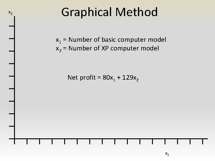
x 2 Graphical Method x 1 = Number of basic computer model x 2 = Number of XP computer model Net profit = 80 x 1 + 129 x 2 x 1

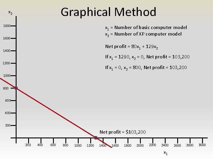
Graphical Method x 2 1800 x 1 = Number of basic computer model x 2 = Number of XP computer model 1600 Net profit = 80 x 1 + 129 x 2 1400 If x 1 = 1290, x 2 = 0, Net profit = 103, 200 1200 If x 1 = 0, x 2 = 800, Net profit = 103, 200 1000 800 600 400 200 Net profit = $103, 200 400 600 800 1000 1200 1400 1600 1800 2000 2200 2400 x 1 2600 2800 3000

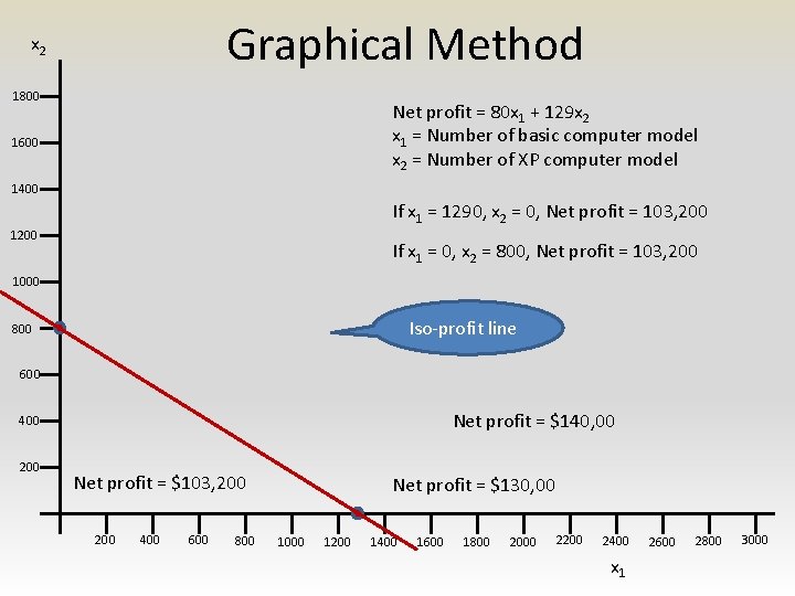
Graphical Method x 2 1800 Net profit = 80 x 1 + 129 x 2 x 1 = Number of basic computer model x 2 = Number of XP computer model 1600 1400 If x 1 = 1290, x 2 = 0, Net profit = 103, 200 1200 If x 1 = 0, x 2 = 800, Net profit = 103, 200 1000 Iso-profit line 800 600 Net profit = $140, 00 400 200 Net profit = $103, 200 400 600 800 Net profit = $130, 00 1000 1200 1400 1600 1800 2000 2200 2400 x 1 2600 2800 3000

Constraints Labor hours constraints Assembly labor Testing labor Basic Model XP Model Hours available 5 hours/unit 6 hours/unit 10, 000 hours 1 hour/unit 2 hours/unit 3, 000 hours Sales constraints Maximum sales/month Basic Model XP Model 600 1200

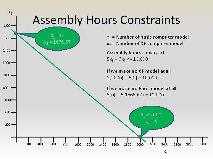
x 2 Assembly Hours Constraints 1800 X 1 = 0, x 2 = 1666. 67 1600 x 1 = Number of basic computer model x 2 = Number of XP computer model 1400 Assembly hours constraint: 5 x 1 + 6 x 2 <= 10, 000 1200 If we make no XP model at all 5(2000) + 6(0) = 10, 000 1800 If we make no Basic model at all 5(0) + 6(1666. 67) = 10, 000 800 600 400 X 1 = 2000, x 2 = 0 200 400 600 800 1000 1200 1400 1600 1800 2000 2200 2400 x 1 2600 2800 3000

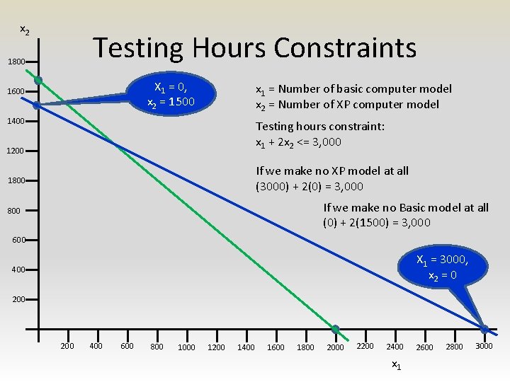
x 2 Testing Hours Constraints 1800 X 1 = 0, x 2 = 1500 1600 x 1 = Number of basic computer model x 2 = Number of XP computer model 1400 Testing hours constraint: x 1 + 2 x 2 <= 3, 000 1200 If we make no XP model at all (3000) + 2(0) = 3, 000 1800 If we make no Basic model at all (0) + 2(1500) = 3, 000 800 600 X 1 = 3000, x 2 = 0 400 200 400 600 800 1000 1200 1400 1600 1800 2000 2200 2400 x 1 2600 2800 3000

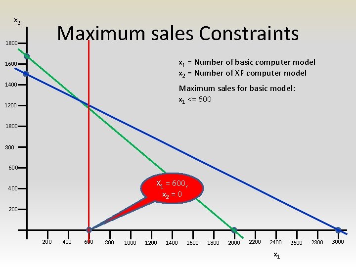
x 2 Maximum sales Constraints 1800 x 1 = Number of basic computer model x 2 = Number of XP computer model 1600 1400 Maximum sales for basic model: x 1 <= 600 1200 1800 600 X 1 = 600, x 2 = 0 400 200 400 600 800 1000 1200 1400 1600 1800 2000 2200 2400 x 1 2600 2800 3000

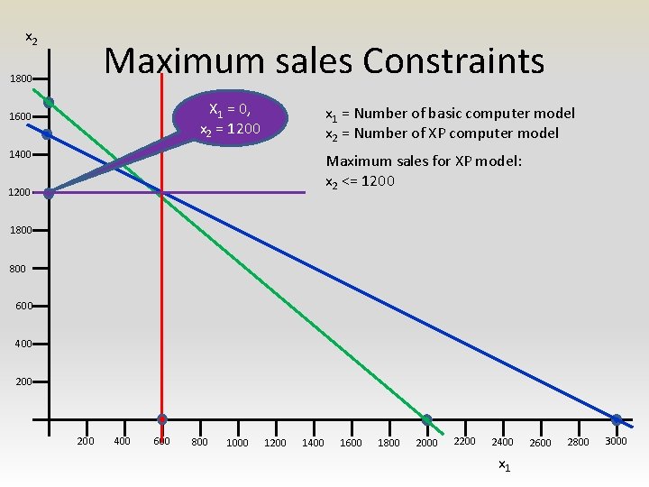
x 2 Maximum sales Constraints 1800 X 1 = 0, x 2 = 1200 1600 x 1 = Number of basic computer model x 2 = Number of XP computer model 1400 Maximum sales for XP model: x 2 <= 1200 1800 600 400 200 400 600 800 1000 1200 1400 1600 1800 2000 2200 2400 x 1 2600 2800 3000

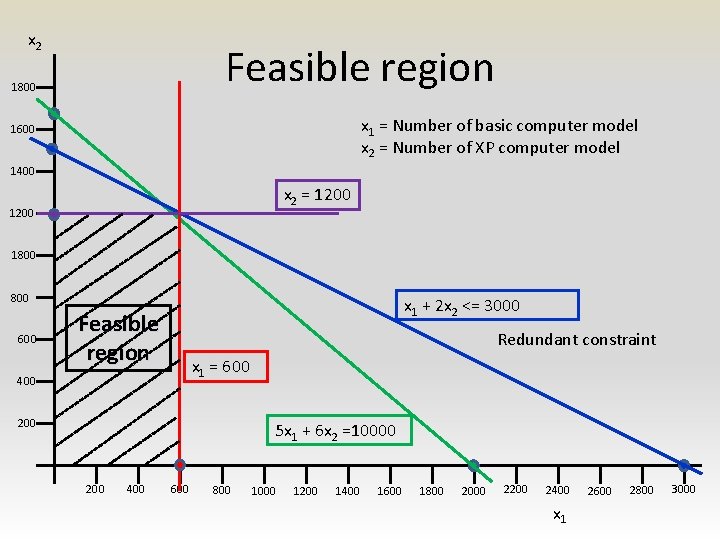
x 2 Feasible region 1800 x 1 = Number of basic computer model x 2 = Number of XP computer model 1600 1400 x 2 = 1200 1800 600 x 1 + 2 x 2 <= 3000 Feasible region Redundant constraint x 1 = 600 400 200 5 x 1 + 6 x 2 =10000 200 400 600 800 1000 1200 1400 1600 1800 2000 2200 2400 x 1 2600 2800 3000

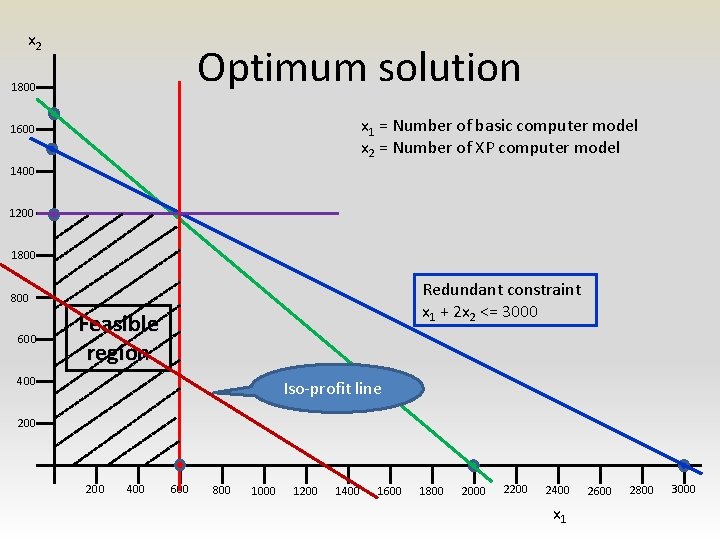
x 2 Optimum solution 1800 x 1 = Number of basic computer model x 2 = Number of XP computer model 1600 1400 1200 1800 Redundant constraint x 1 + 2 x 2 <= 3000 800 600 Feasible region 400 Iso-profit line 200 400 600 800 1000 1200 1400 1600 1800 2000 2200 2400 x 1 2600 2800 3000

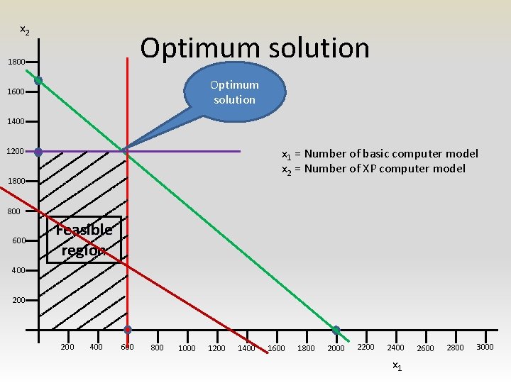
x 2 Optimum solution 1800 Optimum solution 1600 1400 x 1 = Number of basic computer model x 2 = Number of XP computer model 1200 1800 600 Feasible region 400 200 400 600 800 1000 1200 1400 1600 1800 2000 2200 2400 x 1 2600 2800 3000

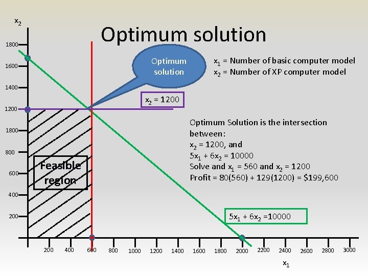
x 2 Optimum solution 1800 x 1 = Number of basic computer model x 2 = Number of XP computer model Optimum solution 1600 1400 x 2 = 1200 Optimum Solution is the intersection between: x 2 = 1200, and 5 x 1 + 6 x 2 = 10000 Solve and x 1 = 560 and x 2 = 1200 Profit = 80(560) + 129(1200) = $199, 600 1800 600 Feasible region 400 5 x 1 + 6 x 2 =10000 200 400 600 800 1000 1200 1400 1600 1800 2000 2200 2400 x 1 2600 2800 3000

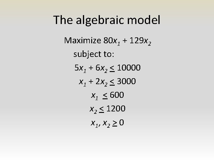
The algebraic model Maximize 80 x 1 + 129 x 2 subject to: 5 x 1 + 6 x 2 < 10000 x 1 + 2 x 2 < 3000 x 1 < 600 x 2 < 1200 x 1 , x 2 > 0

Elements of LP model • Decision variables – The variable whose values must be determined • Objective function – A linear function of decision variables – The value of this function is to be optimized – minimized or maximized • Constraints – Linear functions of the variables – Represents limited resources or minimum requirements

LP requirements • • • Proportionality of variables Additivity of resources Divisibility of variables Non-negativity Linear objective function Linear constraints

Scaling in LP • Poorly scaled model – model contains some very large numbers (e. g. 100, 000 or more) and some very small numbers (e. g. 0. 001 or less) – Solver may erroneously give an error that the linearity conditions are not satisfied • Three remedies for poorly scaled model – Use Automatic Scaling option in Solver/Options – Redefine the units in the model – Change the Precision setting in Solver's Options dialog box to a larger number, such 0. 00001 or 0. 0001. (The default has five zeros. )

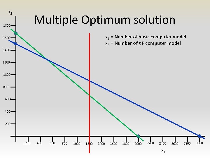
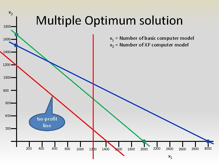
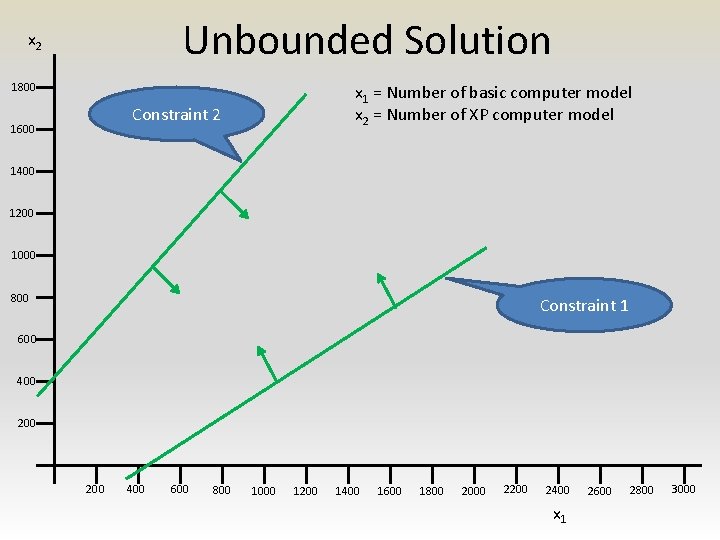
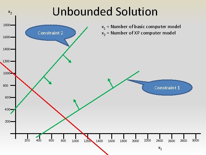
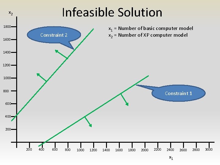
Solutions to LP problem • Feasible solution • Feasible region • Optimal solution – Unique – Multiple – Unbounded

x 2 Multiple Optimum solution 1800 x 1 = Number of basic computer model x 2 = Number of XP computer model 1600 1400 1200 1800 600 400 200 400 600 800 1000 1200 1400 1600 1800 2000 2200 2400 x 1 2600 2800 3000

x 2 Multiple Optimum solution 1800 x 1 = Number of basic computer model x 2 = Number of XP computer model 1600 1400 1200 1800 600 400 Iso-profit line 200 400 600 800 1000 1200 1400 1600 1800 2000 2200 2400 x 1 2600 2800 3000

Unbounded Solution x 2 1800 x 1 = Number of basic computer model x 2 = Number of XP computer model Constraint 2 1600 1400 1200 1000 800 Constraint 1 600 400 200 400 600 800 1000 1200 1400 1600 1800 2000 2200 2400 x 1 2600 2800 3000

Infeasible Solution x 2 1800 x 1 = Number of basic computer model x 2 = Number of XP computer model Constraint 2 1600 1400 1200 1000 800 Constraint 1 600 400 200 400 600 800 1000 1200 1400 1600 1800 2000 2200 2400 x 1 2600 2800 3000

Summary • An LP model may result in – an unique optimum solution – multiple optimum solutions – unbounded feasible region – infeasible region