Chapter 3 Introduction to Linear Programming 2015 Mc

Chapter 3 Introduction to Linear Programming © 2015 Mc. Graw-Hill Education. All rights reserved.

Introduction • Linear programming – Programming means planning – Model contains linear mathematical functions • An application of linear programming – Allocating limited resources among competing activities in the best possible way – Applies to wide variety of situations © 2015 Mc. Graw-Hill Education. All rights reserved. 2

3. 1 Prototype Example • Wyndor Glass Co. – Produces windows and glass doors – Plant 1 makes aluminum frames and hardware – Plant 2 makes wood frames – Plant 3 produces glass and assembles products © 2015 Mc. Graw-Hill Education. All rights reserved. 3

Prototype Example • Company introducing two new products – Product 1: 8 ft. glass door with aluminum frame – Product 2: 4 x 6 ft. double-hung, wood-framed window • Define the problem: What mix of products would be most profitable (determine the production rate of each product to maximize the profit)? – Assuming company could sell as much of either product as could be produced © 2015 Mc. Graw-Hill Education. All rights reserved. 4

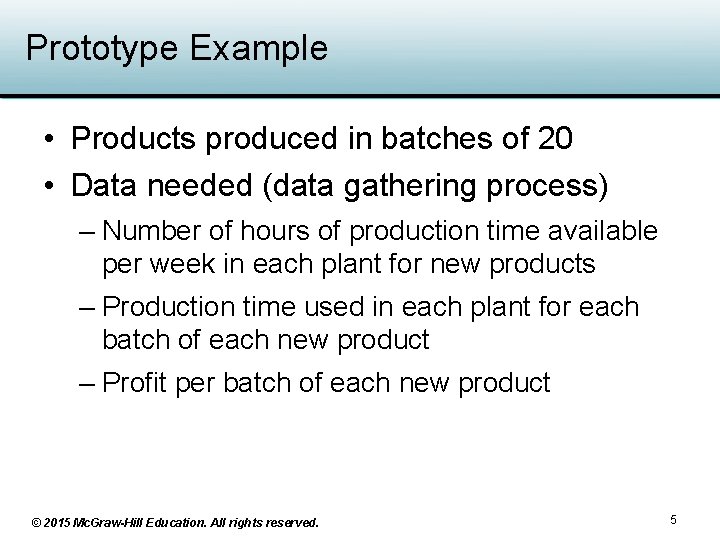
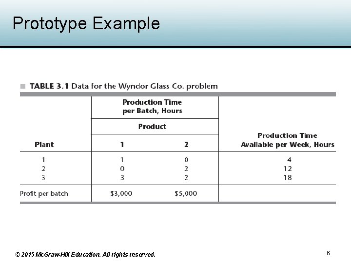
Prototype Example • Products produced in batches of 20 • Data needed (data gathering process) – Number of hours of production time available per week in each plant for new products – Production time used in each plant for each batch of each new product – Profit per batch of each new product © 2015 Mc. Graw-Hill Education. All rights reserved. 5

Prototype Example © 2015 Mc. Graw-Hill Education. All rights reserved. 6

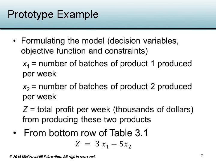
Prototype Example • © 2015 Mc. Graw-Hill Education. All rights reserved. 7

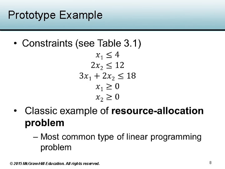
Prototype Example • © 2015 Mc. Graw-Hill Education. All rights reserved. 8

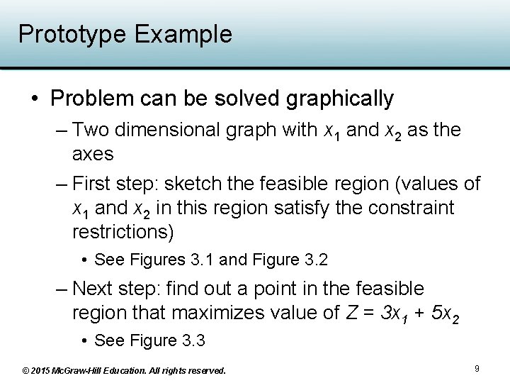
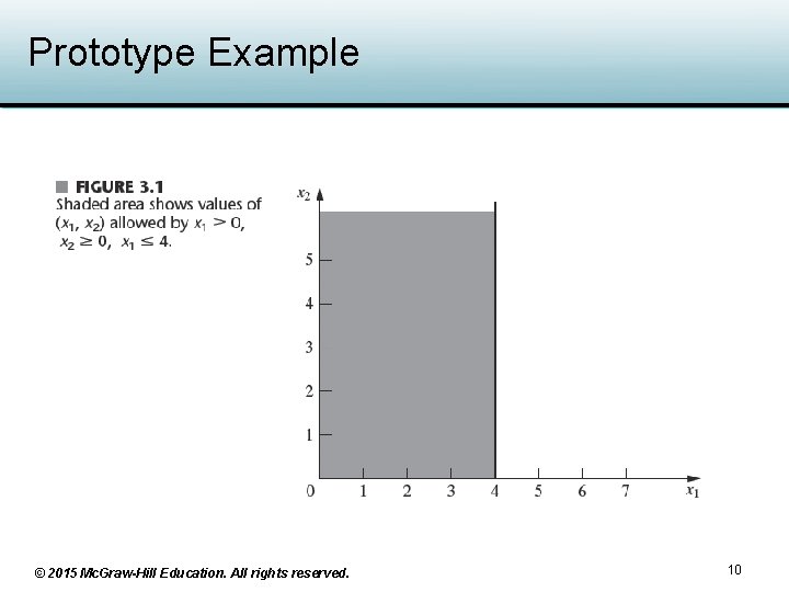
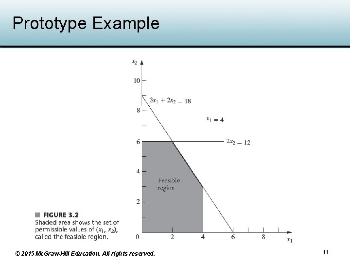
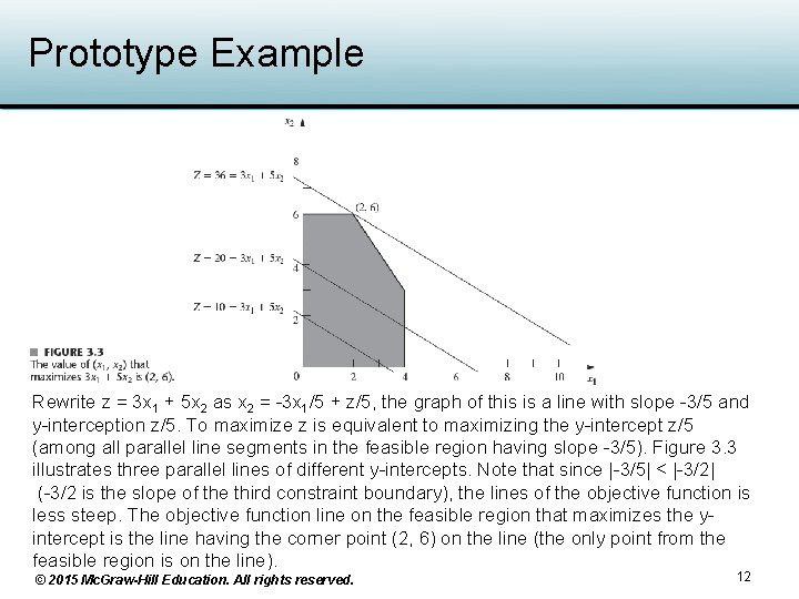
Prototype Example • Problem can be solved graphically – Two dimensional graph with x 1 and x 2 as the axes – First step: sketch the feasible region (values of x 1 and x 2 in this region satisfy the constraint restrictions) • See Figures 3. 1 and Figure 3. 2 – Next step: find out a point in the feasible region that maximizes value of Z = 3 x 1 + 5 x 2 • See Figure 3. 3 © 2015 Mc. Graw-Hill Education. All rights reserved. 9

Prototype Example © 2015 Mc. Graw-Hill Education. All rights reserved. 10

Prototype Example © 2015 Mc. Graw-Hill Education. All rights reserved. 11

Prototype Example Rewrite z = 3 x 1 + 5 x 2 as x 2 = -3 x 1/5 + z/5, the graph of this is a line with slope -3/5 and y-interception z/5. To maximize z is equivalent to maximizing the y-intercept z/5 (among all parallel line segments in the feasible region having slope -3/5). Figure 3. 3 illustrates three parallel lines of different y-intercepts. Note that since |-3/5| < |-3/2| (-3/2 is the slope of the third constraint boundary), the lines of the objective function is less steep. The objective function line on the feasible region that maximizes the yintercept is the line having the corner point (2, 6) on the line (the only point from the feasible region is on the line). © 2015 Mc. Graw-Hill Education. All rights reserved. 12

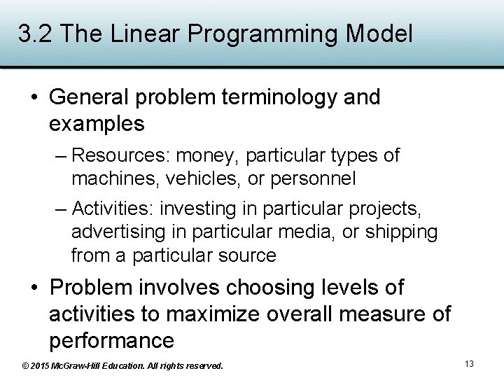
3. 2 The Linear Programming Model • General problem terminology and examples – Resources: money, particular types of machines, vehicles, or personnel – Activities: investing in particular projects, advertising in particular media, or shipping from a particular source • Problem involves choosing levels of activities to maximize overall measure of performance © 2015 Mc. Graw-Hill Education. All rights reserved. 13

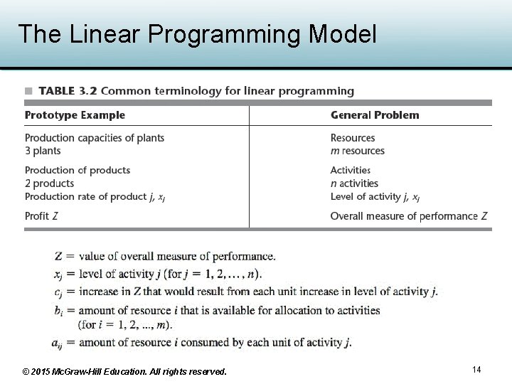
The Linear Programming Model © 2015 Mc. Graw-Hill Education. All rights reserved. 14

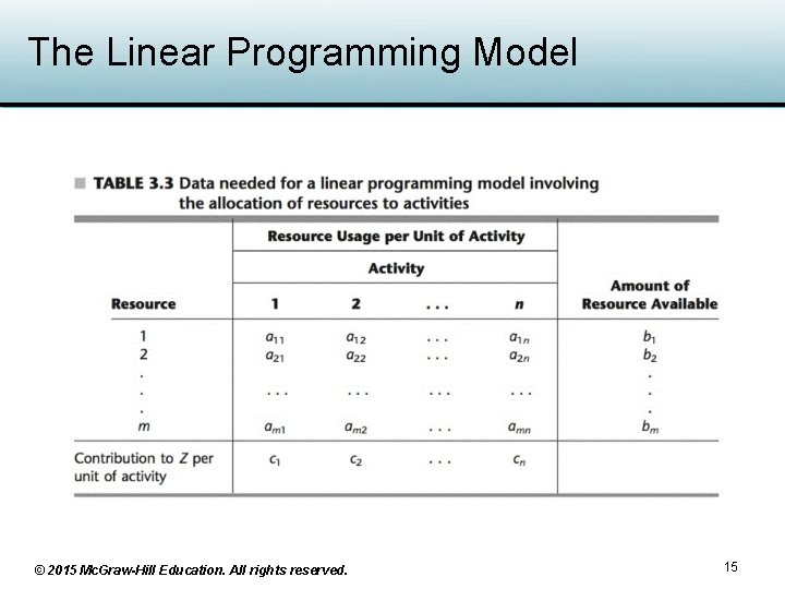
The Linear Programming Model © 2015 Mc. Graw-Hill Education. All rights reserved. 15

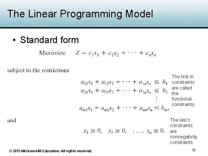
The Linear Programming Model • Standard form The first m constraints are called the functional constraints. The last n constraints are nonnegativity constraints. © 2015 Mc. Graw-Hill Education. All rights reserved. 16

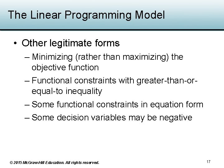
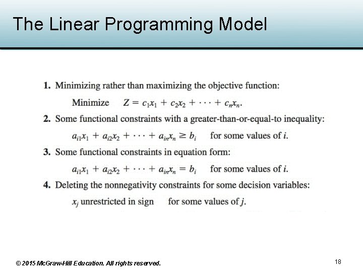
The Linear Programming Model • Other legitimate forms – Minimizing (rather than maximizing) the objective function – Functional constraints with greater-than-orequal-to inequality – Some functional constraints in equation form – Some decision variables may be negative © 2015 Mc. Graw-Hill Education. All rights reserved. 17

The Linear Programming Model © 2015 Mc. Graw-Hill Education. All rights reserved. 18

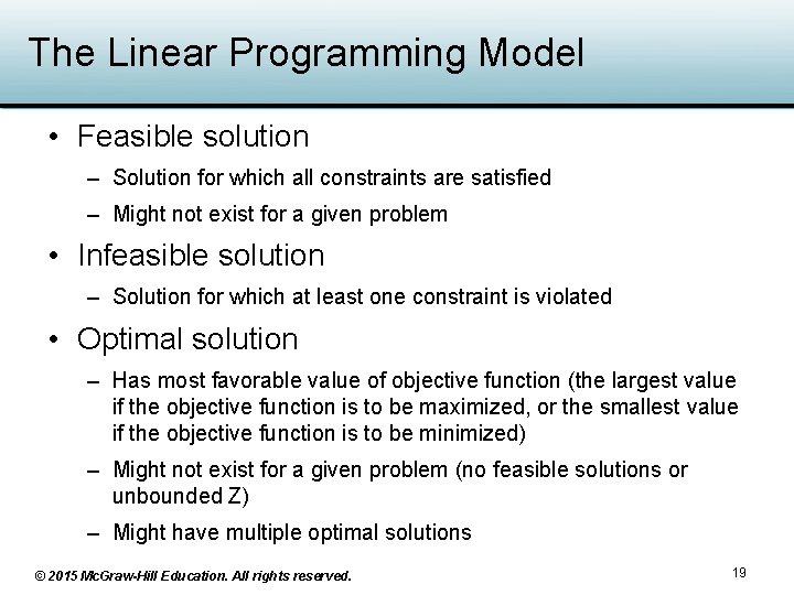
The Linear Programming Model • Feasible solution – Solution for which all constraints are satisfied – Might not exist for a given problem • Infeasible solution – Solution for which at least one constraint is violated • Optimal solution – Has most favorable value of objective function (the largest value if the objective function is to be maximized, or the smallest value if the objective function is to be minimized) – Might not exist for a given problem (no feasible solutions or unbounded Z) – Might have multiple optimal solutions © 2015 Mc. Graw-Hill Education. All rights reserved. 19

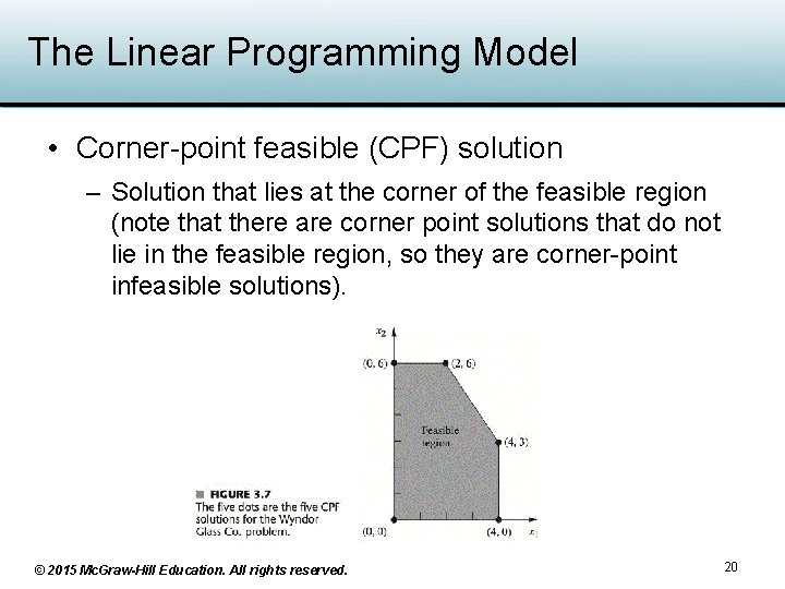
The Linear Programming Model • Corner-point feasible (CPF) solution – Solution that lies at the corner of the feasible region (note that there are corner point solutions that do not lie in the feasible region, so they are corner-point infeasible solutions). © 2015 Mc. Graw-Hill Education. All rights reserved. 20

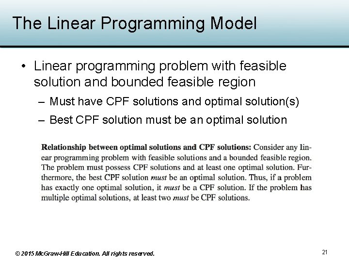
The Linear Programming Model • Linear programming problem with feasible solution and bounded feasible region – Must have CPF solutions and optimal solution(s) – Best CPF solution must be an optimal solution © 2015 Mc. Graw-Hill Education. All rights reserved. 21

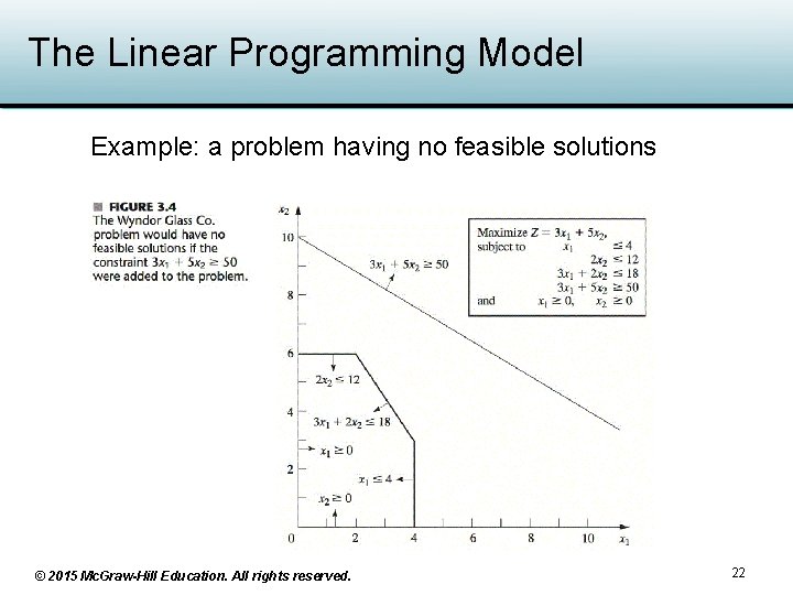
The Linear Programming Model Example: a problem having no feasible solutions © 2015 Mc. Graw-Hill Education. All rights reserved. 22

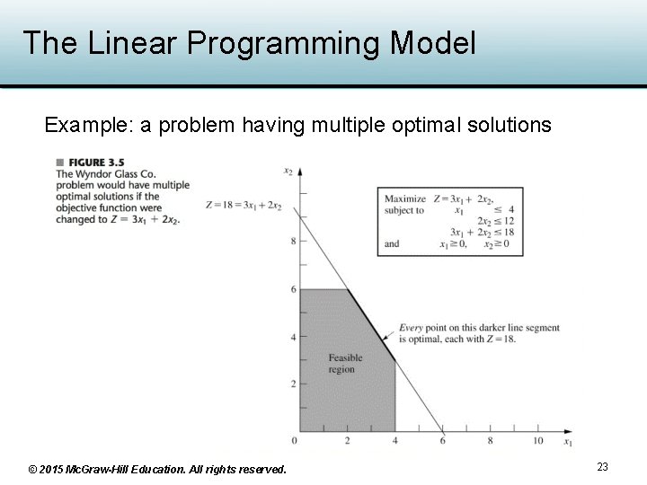
The Linear Programming Model Example: a problem having multiple optimal solutions © 2015 Mc. Graw-Hill Education. All rights reserved. 23

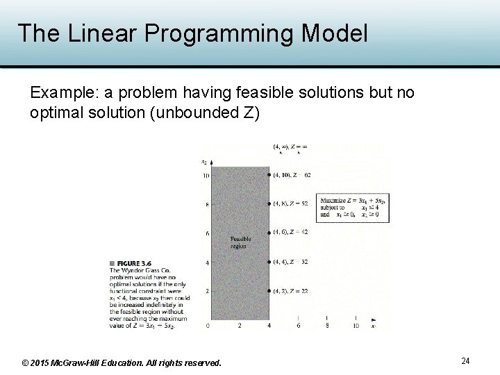
The Linear Programming Model Example: a problem having feasible solutions but no optimal solution (unbounded Z) © 2015 Mc. Graw-Hill Education. All rights reserved. 24

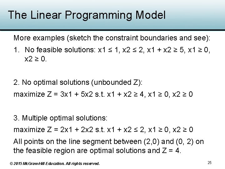
The Linear Programming Model More examples (sketch the constraint boundaries and see): 1. No feasible solutions: x 1 ≤ 1, x 2 ≤ 2, x 1 + x 2 ≥ 5, x 1 ≥ 0, x 2 ≥ 0. 2. No optimal solutions (unbounded Z): maximize Z = 3 x 1 + 5 x 2 s. t. x 1 + x 2 ≥ 4, x 1 ≥ 0, x 2 ≥ 0 3. Multiple optimal solutions: maximize Z = 2 x 1 + 2 x 2 s. t. x 1 + x 2 ≤ 2, x 1 ≥ 0, x 2 ≥ 0 All points on the line segment between (2, 0) and (0, 2) on the feasible region are optimal solutions and Z = 4. © 2015 Mc. Graw-Hill Education. All rights reserved. 25

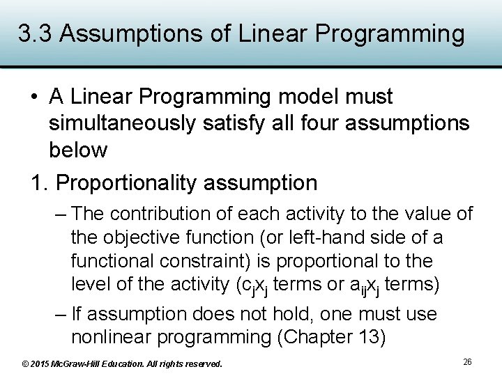
3. 3 Assumptions of Linear Programming • A Linear Programming model must simultaneously satisfy all four assumptions below 1. Proportionality assumption – The contribution of each activity to the value of the objective function (or left-hand side of a functional constraint) is proportional to the level of the activity (cjxj terms or aijxj terms) – If assumption does not hold, one must use nonlinear programming (Chapter 13) © 2015 Mc. Graw-Hill Education. All rights reserved. 26

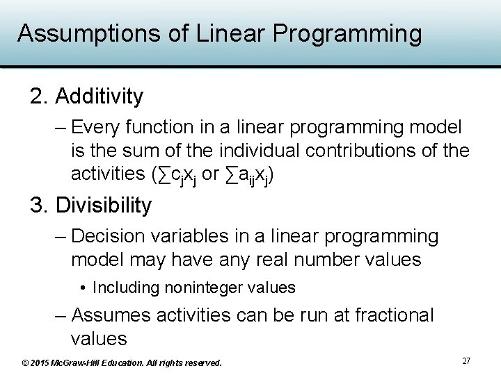
Assumptions of Linear Programming 2. Additivity – Every function in a linear programming model is the sum of the individual contributions of the activities (∑cjxj or ∑aijxj) 3. Divisibility – Decision variables in a linear programming model may have any real number values • Including noninteger values – Assumes activities can be run at fractional values © 2015 Mc. Graw-Hill Education. All rights reserved. 27

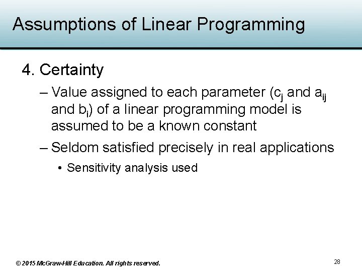
Assumptions of Linear Programming 4. Certainty – Value assigned to each parameter (cj and aij and bi) of a linear programming model is assumed to be a known constant – Seldom satisfied precisely in real applications • Sensitivity analysis used © 2015 Mc. Graw-Hill Education. All rights reserved. 28

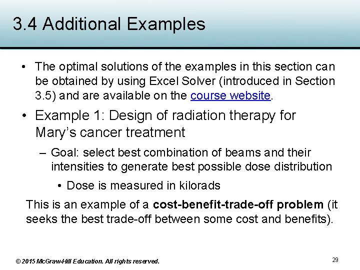
3. 4 Additional Examples • The optimal solutions of the examples in this section can be obtained by using Excel Solver (introduced in Section 3. 5) and are available on the course website. • Example 1: Design of radiation therapy for Mary’s cancer treatment – Goal: select best combination of beams and their intensities to generate best possible dose distribution • Dose is measured in kilorads This is an example of a cost-benefit-trade-off problem (it seeks the best trade-off between some cost and benefits). © 2015 Mc. Graw-Hill Education. All rights reserved. 29

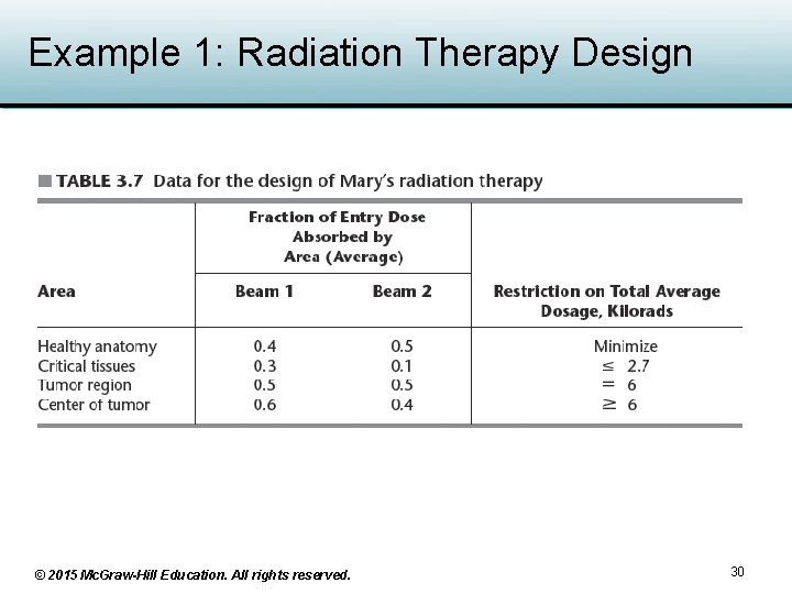
Example 1: Radiation Therapy Design © 2015 Mc. Graw-Hill Education. All rights reserved. 30

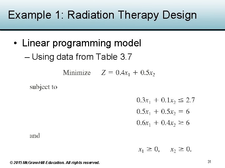
Example 1: Radiation Therapy Design • Linear programming model – Using data from Table 3. 7 © 2015 Mc. Graw-Hill Education. All rights reserved. 31

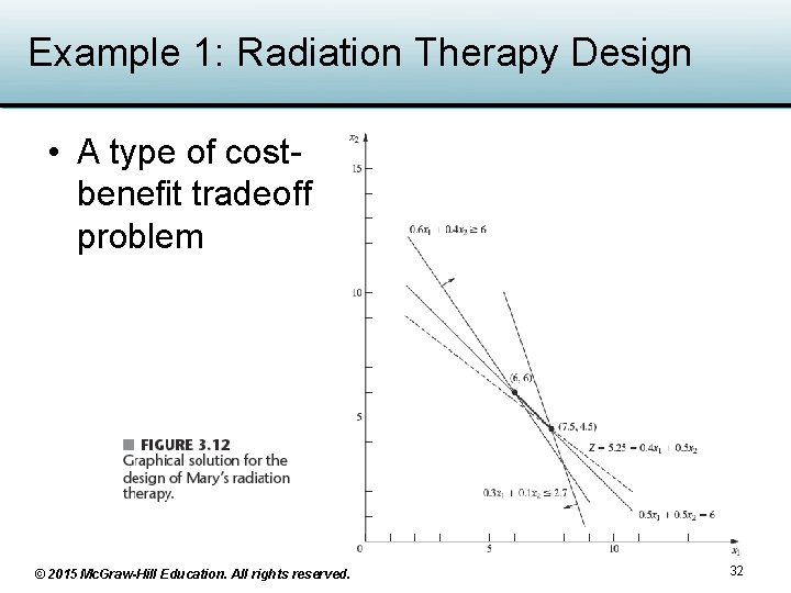
Example 1: Radiation Therapy Design • A type of costbenefit tradeoff problem © 2015 Mc. Graw-Hill Education. All rights reserved. 32

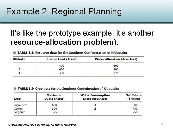
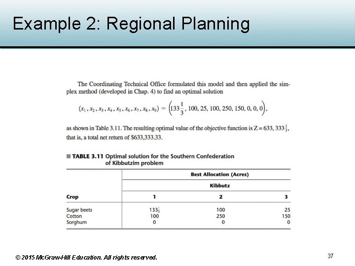
Example 2: Regional Planning It’s like the prototype example, it’s another resource-allocation problem). © 2015 Mc. Graw-Hill Education. All rights reserved. 33

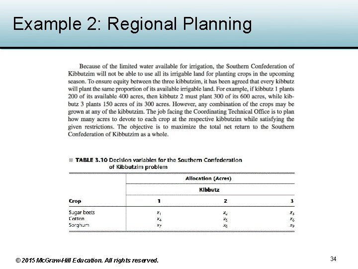
Example 2: Regional Planning © 2015 Mc. Graw-Hill Education. All rights reserved. 34

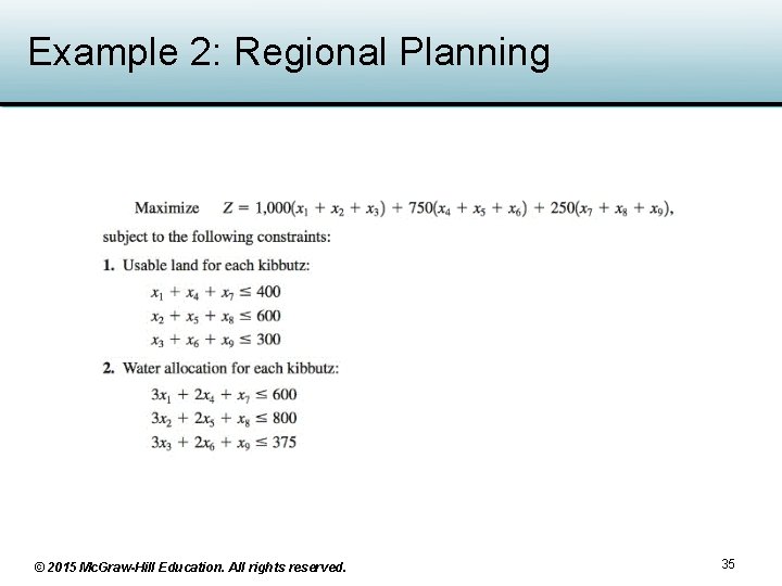
Example 2: Regional Planning © 2015 Mc. Graw-Hill Education. All rights reserved. 35

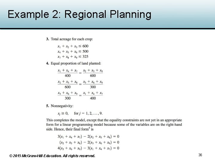
Example 2: Regional Planning © 2015 Mc. Graw-Hill Education. All rights reserved. 36

Example 2: Regional Planning © 2015 Mc. Graw-Hill Education. All rights reserved. 37

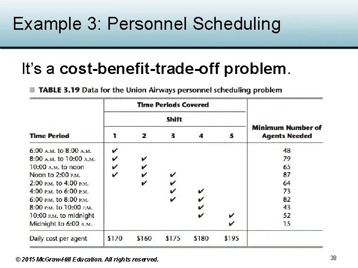
Example 3: Personnel Scheduling It’s a cost-benefit-trade-off problem. © 2015 Mc. Graw-Hill Education. All rights reserved. 38

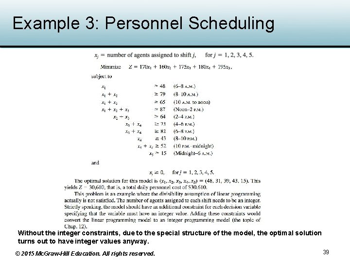
Example 3: Personnel Scheduling Without the integer constraints, due to the special structure of the model, the optimal solution turns out to have integer values anyway. © 2015 Mc. Graw-Hill Education. All rights reserved. 39

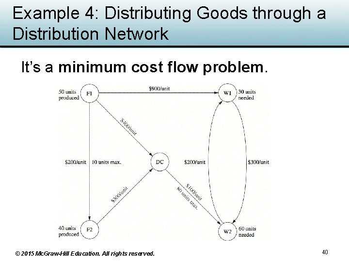
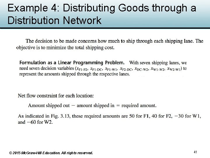
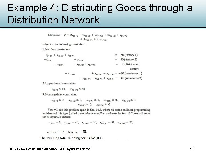
Example 4: Distributing Goods through a Distribution Network It’s a minimum cost flow problem. © 2015 Mc. Graw-Hill Education. All rights reserved. 40

Example 4: Distributing Goods through a Distribution Network © 2015 Mc. Graw-Hill Education. All rights reserved. 41

Example 4: Distributing Goods through a Distribution Network © 2015 Mc. Graw-Hill Education. All rights reserved. 42

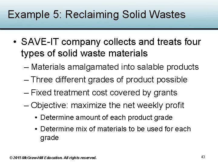
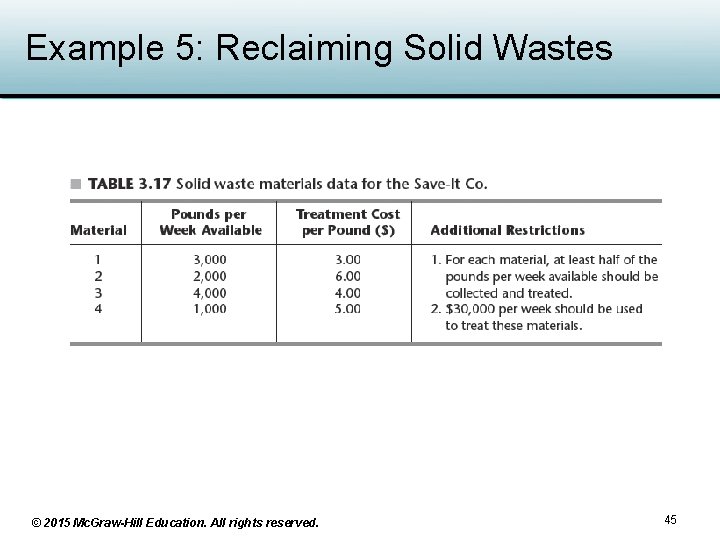
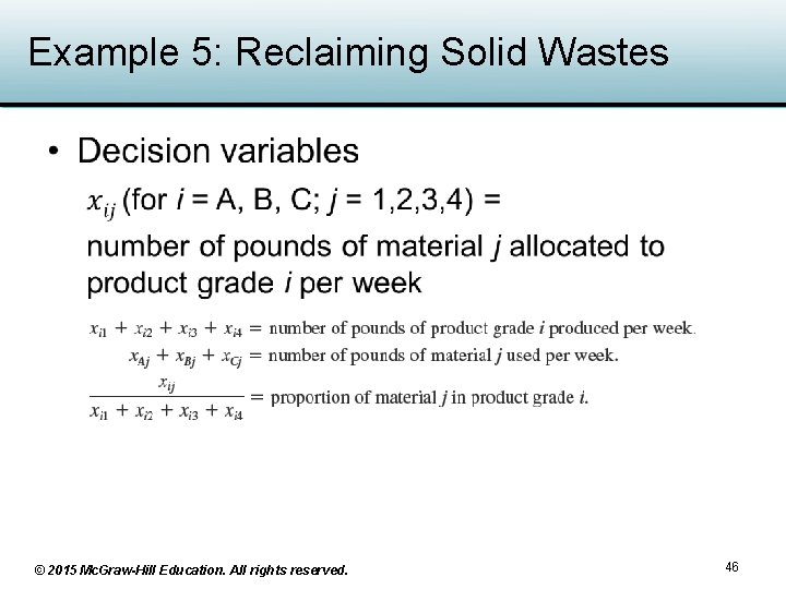
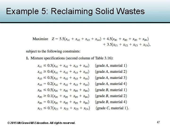
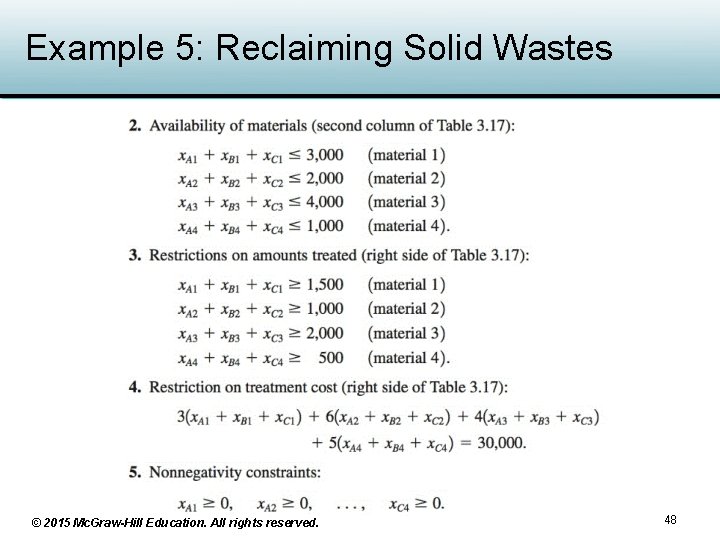
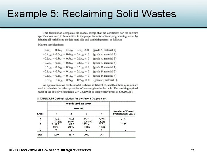
Example 5: Reclaiming Solid Wastes • SAVE-IT company collects and treats four types of solid waste materials – Materials amalgamated into salable products – Three different grades of product possible – Fixed treatment cost covered by grants – Objective: maximize the net weekly profit • Determine amount of each product grade • Determine mix of materials to be used for each grade © 2015 Mc. Graw-Hill Education. All rights reserved. 43

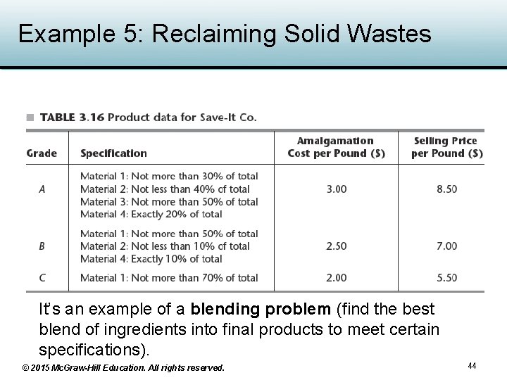
Example 5: Reclaiming Solid Wastes It’s an example of a blending problem (find the best blend of ingredients into final products to meet certain specifications). © 2015 Mc. Graw-Hill Education. All rights reserved. 44

Example 5: Reclaiming Solid Wastes © 2015 Mc. Graw-Hill Education. All rights reserved. 45

Example 5: Reclaiming Solid Wastes • © 2015 Mc. Graw-Hill Education. All rights reserved. 46

Example 5: Reclaiming Solid Wastes © 2015 Mc. Graw-Hill Education. All rights reserved. 47

Example 5: Reclaiming Solid Wastes © 2015 Mc. Graw-Hill Education. All rights reserved. 48

Example 5: Reclaiming Solid Wastes © 2015 Mc. Graw-Hill Education. All rights reserved. 49

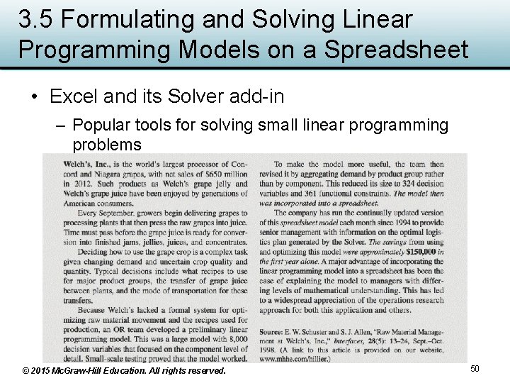
3. 5 Formulating and Solving Linear Programming Models on a Spreadsheet • Excel and its Solver add-in – Popular tools for solving small linear programming problems © 2015 Mc. Graw-Hill Education. All rights reserved. 50

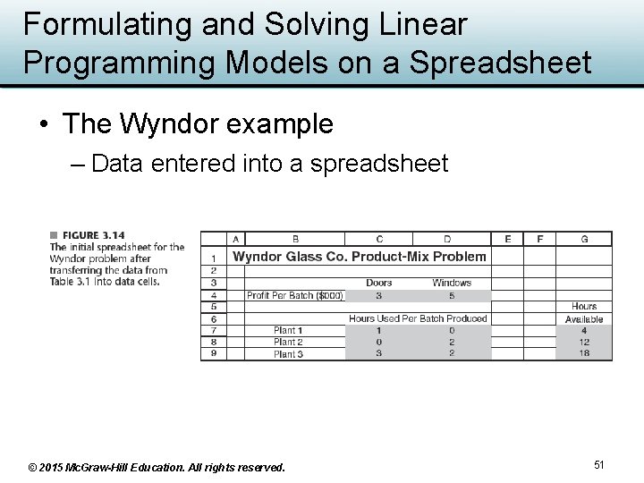
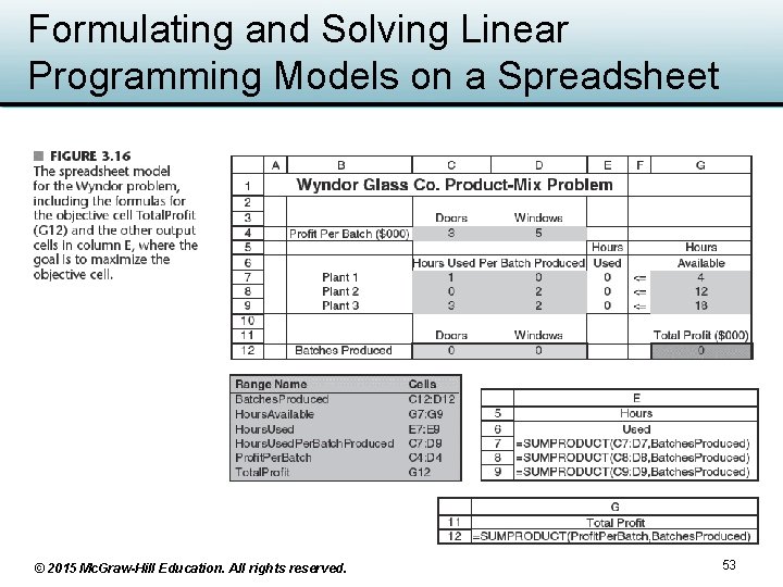
Formulating and Solving Linear Programming Models on a Spreadsheet • The Wyndor example – Data entered into a spreadsheet © 2015 Mc. Graw-Hill Education. All rights reserved. 51

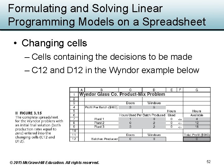
Formulating and Solving Linear Programming Models on a Spreadsheet • Changing cells – Cells containing the decisions to be made – C 12 and D 12 in the Wyndor example below © 2015 Mc. Graw-Hill Education. All rights reserved. 52

Formulating and Solving Linear Programming Models on a Spreadsheet © 2015 Mc. Graw-Hill Education. All rights reserved. 53

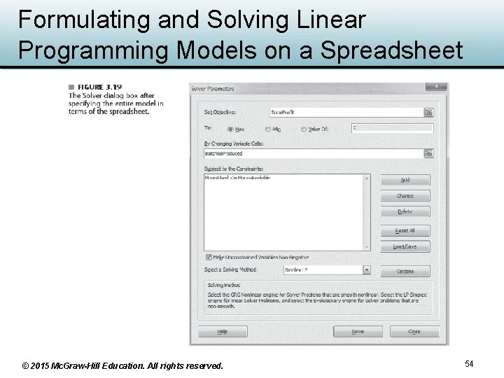
Formulating and Solving Linear Programming Models on a Spreadsheet © 2015 Mc. Graw-Hill Education. All rights reserved. 54

3. 6 Formulating Very Large Linear Programming Models • Actual linear programming models – Can have hundreds or thousands of functional constraints – Number of decision variables may also be very large • Modeling language – Used to formulate very large models in practice – Expedites model management tasks © 2015 Mc. Graw-Hill Education. All rights reserved. 55

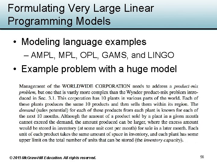
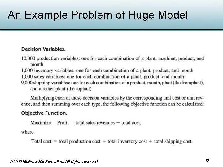
Formulating Very Large Linear Programming Models • Modeling language examples – AMPL, OPL, GAMS, and LINGO • Example problem with a huge model © 2015 Mc. Graw-Hill Education. All rights reserved. 56

An Example Problem of Huge Model © 2015 Mc. Graw-Hill Education. All rights reserved. 57

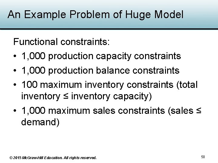
An Example Problem of Huge Model Functional constraints: • 1, 000 production capacity constraints • 1, 000 production balance constraints • 100 maximum inventory constraints (total inventory ≤ inventory capacity) • 1, 000 maximum sales constraints (sales ≤ demand) © 2015 Mc. Graw-Hill Education. All rights reserved. 58

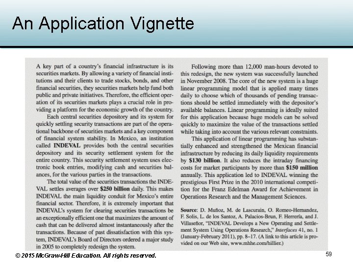
An Application Vignette © 2015 Mc. Graw-Hill Education. All rights reserved. 59

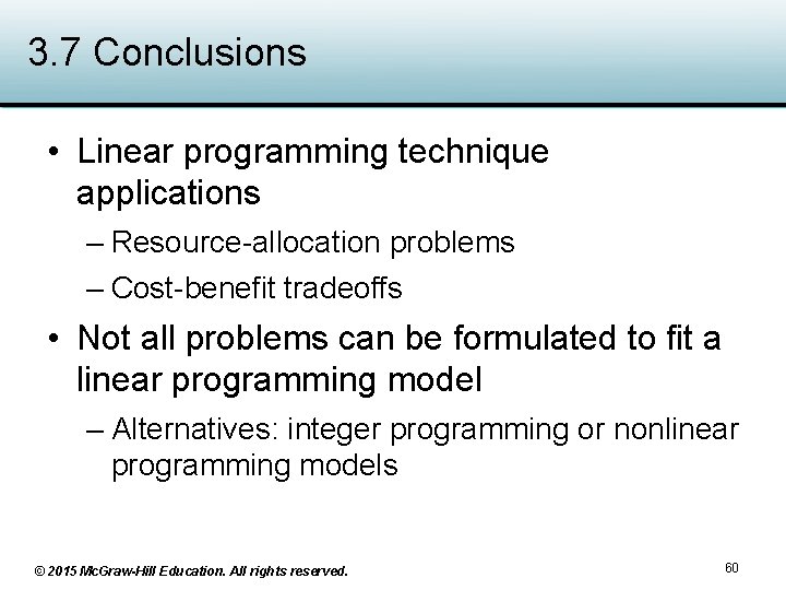
3. 7 Conclusions • Linear programming technique applications – Resource-allocation problems – Cost-benefit tradeoffs • Not all problems can be formulated to fit a linear programming model – Alternatives: integer programming or nonlinear programming models © 2015 Mc. Graw-Hill Education. All rights reserved. 60