Chapter 3 Graphics Output Primitives 2010 1 Chapter


 gl. Load.")

 2010")
![int point 1 [ ] = {50, 100} ; int point 2 [](https://slidetodoc.com/presentation_image_h/32490732d849abbc7f1001a8edfffcbd/image-7.jpg "int point 1 [ ] = {50, 100} ; int point 2 [")

; gl. Vertex 2 iv (p 1); gl.")
; gl. Vertex 2 iv (p 1); gl. Vertex 2 iv (p")


 produced when a line is generated as a")
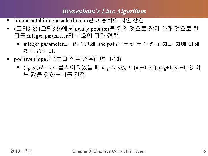
 § x, y의 계산을 기본으로 한 scan-conversion line")


 = (xk+1)2 + (yk-1/2)2")

 = ((xk+1)+1)2 + (yk+1 -1/2)2 - r 2")


 (-x, -y) (x,")


")


 두 번째 방법으로는, plane normal의 성분을 vector cross product 계산으 로 구함 §")


- Slides: 56
Chapter 3. Graphics Output Primitives 2010 -1학기 Chapter 3. Graphics Output Primitives 1
Point and Lines § point plotting § CRT monitor의 경우: electron beam에 의해 선택된 위치의 스크린 형광 체가 빛을 발하여 나타냄 § random-scan (vector) system의 경우: 디스플레이 리스트에 point-plotting instructions와 좌표값이 저장됨 § black and white system: frame buffer내 스크린위치의 bit value를 1로 세트 하여 한 점을 나타냄 § RGB system: frame buffer를 스크린 픽셀위치에 디스플레이 될 color intensity로 채움 2010 -1학기 Chapter 3. Graphics Output Primitives 2
§ Line drawing § 두 endpoints를 연결하는 line path위의 중간점을 계산하여 나타냄 § 스크린 위치는 정수로 표현되므로 plotted position은 두 끝점을 연결하 는 실제적인 선분에 근접하는 선을 나타내게 됨 § stair step appearance가 생김 (jaggies), low resolution일 경우 현저하게 나타남 § high-resolution systems에서 디스플레이 하거나 § line path에 따라 픽셀의 intensity를 조정하여 raster lines를 매끄 럽게 만듦 § frame buffer내 column x, scanline y의 위치에 intensity value 를 넣는 것을 § set. Pixel (x, y) § retrieve는 get. Pixel (x, y, color) 2010 -1학기 Chapter 3. Graphics Output Primitives 3
§ Two-Dimensional World-Coordinate Reference Frame in Open. GL gl. Matrix. Mode (GL_PROJECTION) gl. Load. Indentity ( ); glu. Ortho 2 D (xmin, xmax, ymin, ymax); => orthogonal projection § Open. GL point functions gl. Begin (GL_POINTS); gl. Vertex 2 i (50, 100); gl. Vertex 2 i (75, 150); gl. Vertex 2 i (100, 200); gl. End ( ); 2010 -1학기 Chapter 3. Graphics Output Primitives 4
Figure 3 -2 World coordinate limits for a display window, as specified in the gl. Ortho 2 D function 2010 -1학기 Chapter 3. Graphics Output Primitives 5
Figure 3 -3 Display of three point positions generated with gl. Begin (GL_POINTS) 2010 -1학기 Chapter 3. Graphics Output Primitives 6
int point 1 [ ] = {50, 100} ; int point 2 [ ] = {75, 150}; int point 3 [ ] = {100, 200} ; gl. Begin (GL_POINTS); gl. Vertex 2 iv (point 1); gl. Vertex 2 iv (point 2); gl. Vertex 2 iv (point 3); gl. End ( ); gl. Begin (GL_POINTS) ; gl. Vertex 3 f (-78. 05, 909. 72, 14. 60); gl. Vertex 3 f (261. 91, -5200. 67, 188. 33); gl. End ( ); 2010 -1학기 Chapter 3. Graphics Output Primitives 7
class wc. Pt 2 D { public : GLFLoat x, y; } ; wc. Pt 2 D point. Pos; point. Pos. x = 120. 75; point. Pos. y = 45. 30; gl. Begin (GL_POINTS) ; gl. Vertex 2 f (point. Pos. x, point. Pos. y); gl. End ( ); 2010 -1학기 Chapter 3. Graphics Output Primitives 8
Open. GL Line Functions gl. Begin (GL_LINES); gl. Vertex 2 iv (p 1); gl. Vertex 2 iv (p 2); gl. Vertex 2 iv (p 3); gl. Vertex 2 iv (p 4); gl. Vertex 2 iv (p 5); gl. End ( ); gl. Begin (GL_LINE_STRIP); gl. Vertex 2 iv (p 1); gl. Vertex 2 iv (p 2); gl. Vertex 2 iv (p 3); gl. Vertex 2 iv (p 4); gl. Vertex 2 iv (p 5); gl. End ( ); 2010 -1학기 Chapter 3. Graphics Output Primitives 9
gl. Begin (GL_LINE_LOOP); gl. Vertex 2 iv (p 1); gl. Vertex 2 iv (p 2); gl. Vertex 2 iv (p 3); gl. Vertex 2 iv (p 4); gl. Vertex 2 iv (p 5); gl. End ( ); 2010 -1학기 Chapter 3. Graphics Output Primitives 10
Figure 3 -4 Line segments that can be displayed in Open. GL using a list of five endpoint coordinates 2010 -1학기 Chapter 3. Graphics Output Primitives 11
Line-Drawing Algorithm § Cartesian slope-intercept equation for a straight line § y = m x + b로 나타냄 (m: slope, b: y-intercept) § 두 점 (x 1, y 1), (x 2, y 2)가 주어졌을 때 slope m과 intercept b는 y 2 - y 1 m = x 2 - x 1 b = y 1 - m * x 1 § 마찬가지로 x interval, y interval은 y = m x x = y / m 2010 -1학기 Chapter 3. Graphics Output Primitives 12
Figure 3 -5 Stair-step effect (jaggies) produced when a line is generated as a series of pixel postions 2010 -1학기 Chapter 3. Graphics Output Primitives 13
DDA Algorithm (Digital Differential Analyzer Algorithm) § x, y의 계산을 기본으로 한 scan-conversion line algorithm § positive slope인 선으로 slope가 1보다 작거나 같을 때: x interval을 단위 1로 하고 y값을 구한다. § yk+1 = yk + m § positive slope가 1보다 큰 경우엔 x, y의 역할을 바꾸어 y interval을 단위 1로 하고 x 값을 구한다. § xk+1 = xk + 1/m § 선분 생성의 starting point가 오른쪽에서부터라면 § yk+1 = yk – m § xk+1 = xk - 1/m 2010 -1학기 Chapter 3. Graphics Output Primitives 14
2010 -1학기 Chapter 3. Graphics Output Primitives 15
Figure 3 -8 A section of a display screen where a straight line segment is to be plotted 13 12 11 10 10 11 12 13 2010 -1학기 Chapter 3. Graphics Output Primitives 17
Figure 3 -9 A section of a display screen where a negative slope line segment is to be plotted 50 49 48 50 51 52 53 2010 -1학기 Chapter 3. Graphics Output Primitives 18
Figure 3 -10 A section of the screen grid showing a pixel 2010 -1학기 Chapter 3. Graphics Output Primitives 19
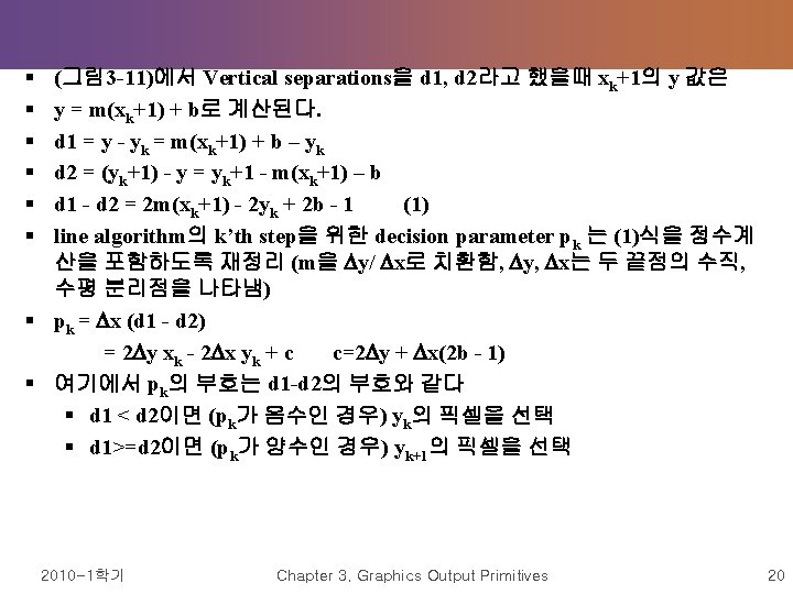
Figure 3 -11 Vertical distances between pixel positions and the line y coordinate at sampling position xk+1 yk+1 d 2 y d 1 yk xk + 1 2010 -1학기 Chapter 3. Graphics Output Primitives 21
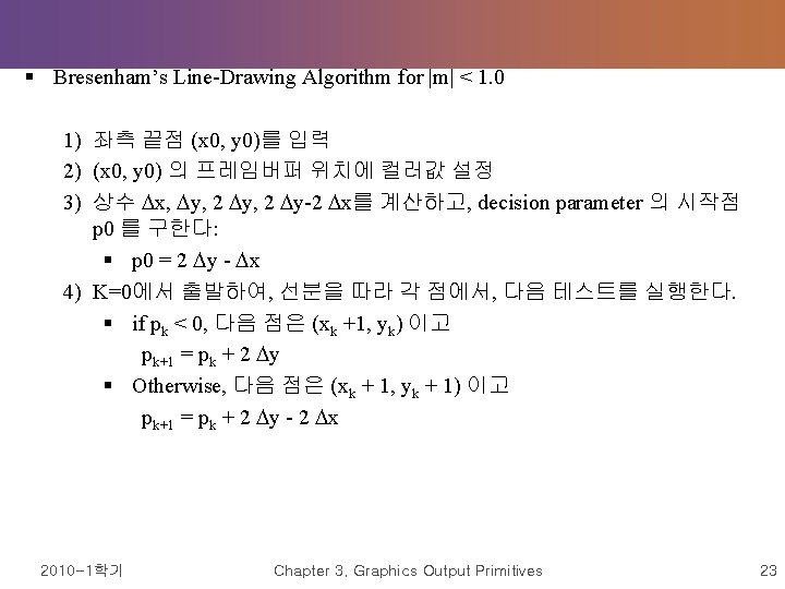
§ incremental integer calculations를 이용하여 연속적으로 decision parameter의 값을 구하기 위해 § step k+1에서 Pk+1 = 2 y xk+1 - 2 x yk+1 + c 이므로 § Pk+1 - Pk = 2 y ( xk+1 - xk) - 2 x (yk+1 - yk)이 얻어짐 § 여기에서 xk+1 = xk + 1이므로 § pk+1 = pk + 2 y - 2 x (yk+1 - yk) 이 됨 § starting pixel position이 (x 0, y 0)이면 § 위의 식 pk = 2 y xk - 2 x yk + c c=2 y + x(2 b - 1) 에서 § p 0 = 2 y - x 가 된다. 2010 -1학기 Chapter 3. Graphics Output Primitives 22
Loading the frame buffer § frame-buffer array가 row-major order로 addressing되고 pixel position은 lowerleft corner에서 (0, 0)에서 출발하여 top-right corner에서 (xmax, ymax)가 된다고 하면 § pixel position (x, y)에 대한 frame-buffer bit address는 § addr(x, y) = addr(0, 0) + y(xmax + 1) +x 2010 -1학기 Chapter 3. Graphics Output Primitives 24
Figure 3 -14 Pixel screen positions stored linearly in row-major order within the frame buffer ymax screen (x, y) 0 0 xmax …. . Frame Buffer …. . . (0, 0) (0, 1) (2, 0) (xmax, 0) (0, 1) addr(x, y) (xmax, ymax) 2010 -1학기 Chapter 3. Graphics Output Primitives 25
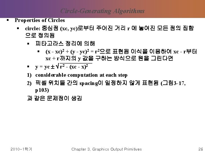
Figure 3 -17 Upper half of a circle plotted with Eq. 3 -27 and with (xc, yc) = (0, 0) 2010 -1학기 Chapter 3. Graphics Output Primitives 28
Figure 3 -18 Symmetry of a circle 2010 -1학기 Chapter 3. Graphics Output Primitives 30
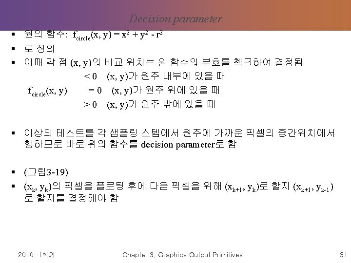
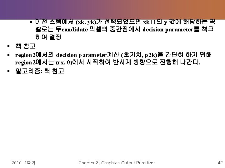
§ decision parameter는 다음과 같다 § pk = fcircle(xk+1, yk-1/2) = (xk+1)2 + (yk-1/2)2 - r 2 § If pk < 0, § Midpoint 가 원 내부에 존재하므로, yk 가 원주에 더 가까우므로 yk 선택 § Otherwise, § Midpoint 가 원 외부 혹은 원주에 존재하며, 이 때는 yk-1 선택 2010 -1학기 Chapter 3. Graphics Output Primitives 32
Figure 3 -19 Midpoint between candidate pixels at sampling position xk+1 along a circular path x 2 + y 2 - r 2 = 0 yk Midpoint yk - 1 xk 2010 -1학기 xk + 1 xk + 2 Chapter 3. Graphics Output Primitives 33
§ pk+1 = fcircle(xk+1+1, yk+1 -1/2) = ((xk+1)+1)2 + (yk+1 -1/2)2 - r 2 § pk+1 = pk + 2(xk+1) + (y 2 k+1 – y 2 k) – (yk+1 – yk) + 1 § yk+1 은 pk 의 부호에 따라 yk 혹은 yk-1 § pk+1 을 얻기 위한 증가분은 § pk가 음수이면 2 xk+1+1 § 아니면 2 xk+1+1 – 2 yk+1 § 2 xk+1 = 2 xk+2 § 2 yk+1 = 2 yk-2 § Decision parameter 의 초기값 p 0 = fcirc(1, r – ½) = 1 + (r – ½)2 – r 2 혹은 p 0 = 5/4 - r 2010 -1학기 Chapter 3. Graphics Output Primitives 34
Midpoint Circle Algorithm 2010 -1학기 Chapter 3. Graphics Output Primitives 35
2010 -1학기 Chapter 3. Graphics Output Primitives 36
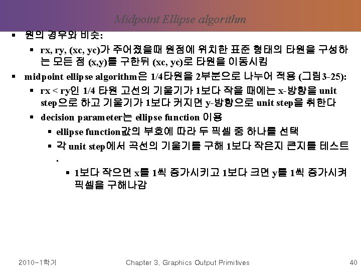
Ellipse-Generating Algorithms § Properties of Ellipses § 타원의 정의 : 두개 정점으로부터의 거리의 합이 일정한 모든 점의 집합 § d 1 + d 2 = constant, 즉 § (x - x 1)2 + (y - y 2)2 + (x - x 2)2 + (y - y 2)2 = constant -> Ax 2 + By 2 + Cxy + Dx + Ey + F = 0 § 타원의 두 축이 x, y축에 평행할 경우엔 타원의 식이 간단하게 됨 § 2010 -1학기 x - xc rx 2 + y - yc 2 = 1 ry Chapter 3. Graphics Output Primitives 37
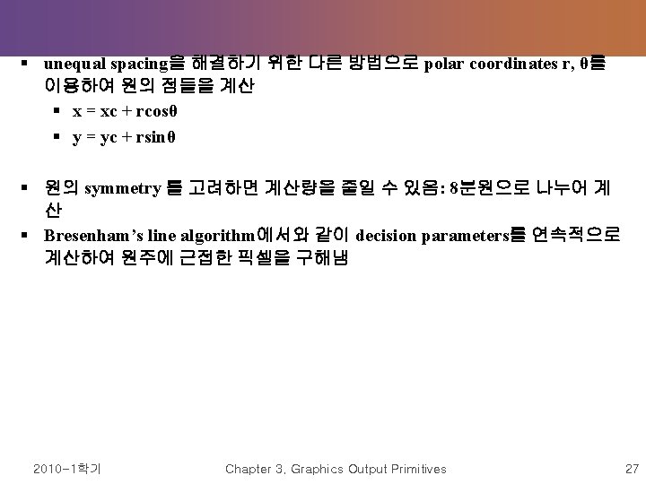
§ polar coordinates r, 를 이용하면 § x = xc + rx cos § y = yc + ry sin § 타원의 특성: 4분원 사이에 대칭 현상으로 원과 다름 (그림 3 -24) 2010 -1학기 Chapter 3. Graphics Output Primitives 38
Figure 3 -24 Symmetry of an ellipse 2010 -1학기 (-x, y) (-x, -y) (x, -y) Chapter 3. Graphics Output Primitives 39
Figure 3 -25 Ellipse processing regions Region 1 Slope = -1 Region 2 2010 -1학기 Chapter 3. Graphics Output Primitives 41
Other Curves § Polynomials and Spline curves § n차 polynomial function y = ak xk = a 0 + a 1 x +. . . + anxn § object shape, animation path 등에 유용 § curve fitting의 한 방법으로 cubic polynomial curve section구성 § 각 curve section을 파라미터 형태의 cubic polynomial curve section으 로 표현 § x = ax 0 + ax 1 u + ax 2 u 2 + ax 3 u 3 § y = ay 0 + ay 1 u + ay 2 u 2 + ay 3 u 3 § 파라미터 u는 0부터 1까지 변화함 § u의 계수 값은 boundary conditions으로 구해짐 1) 두개 인접한 curve는 경계점에서 같은 좌표치를 갖는다. 2) 경계점에서 두 곡선의 기울기가 같다. -> 연속적이고 매끄 러운 곡선 형성에 필요한 조건 2010 -1학기 Chapter 3. Graphics Output Primitives 43
§ spline curve: 이상과 같이 polynomial 조각들로 구성된 연속적 곡선을 말함 (그림 3 -32) 2010 -1학기 Chapter 3. Graphics Output Primitives 44
Figure 3 -32 A Spline curve formed with individual cubic polynomial sections 2010 -1학기 Chapter 3. Graphics Output Primitives 45
Polygon Tables § geometric tables 와 attribute tables로 구성 § geometric tables는 vertex coordinates 와 polygon surfaces의 spatial orientation을 나타내기 위한 파라미터들로 구성되어 있다. § attribute tables엔 물체의 transparency의 정도, surface reflecitivity, texture characteristics등을 위한 파라미터들을 가지고 있다. § geometric data를 위해선 § vertex table: 각 vertex의 coordinate values를 가짐 § edge table: 각 polygon edge의 vertex를 위한 포인터로 구성 § polygon table로 구성: edge table의 포인터로 구성 2010 -1학기 Chapter 3. Graphics Output Primitives 46
Figure 3 -50 Geometric data table representation for two adjacent polygon surfaces V 1 E 3 S 1 V 2 Vertex table V 1: x 1, y 1, z 1 V 2: x 2, y 2, z 2 V 3: x 3, y 3, z 3 V 4: x 4, y 4, z 4 V 5: x 5, y 5, z 5 2010 -1학기 E 2 E 6 S 2 V 3 E 4 Edge table V 5 E 5 V 4 E 1: V 1, V 2 E 2: V 2, V 3 E 3: V 3, V 1 E 4: V 3, V 4 E 5: V 4, V 5 E 6: V 5, V 1 Polygon-Surface table S 1: E 1, E 2, E 3 S 2: E 3, E 4, E 5 E 6 Chapter 3. Graphics Output Primitives 47
§ extra information을 추가하기도 함 § edge table에 polygon table의 포인터를 추가 § edge slope, 각 polygon의 coordinate extents: § edge slope나 bounding-box info는 surface rendering에 이용되고 coordinate extents는 visible-surface determination algorithm에 이용됨 2010 -1학기 Chapter 3. Graphics Output Primitives 48
§ 그래픽스 패키지의 error checking § 모든 vertex는 적어도 two edges의 endpoint § 모든 edge는 적어도 한 polygon의 부분 § 모든 polygon은 closed § 모든 polygon은 적어도 one shared edge를 가짐 § edge table이 polygon 포인터를 가지면 polygon pointer에 의해 reference 되는 edge들은 거꾸로 polygon pointer를 갖는다. 2010 -1학기 Chapter 3. Graphics Output Primitives 49
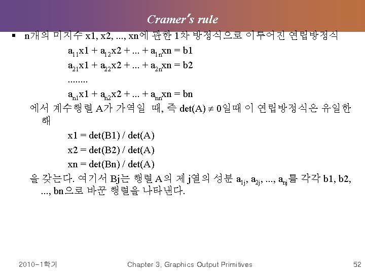
Plane Equations § 3차원 물체의 디스플레이를 위해선 § 모델링, world coordinates에서 viewing coordinates로 다시 device coordinates등의 transformation이 필요하고 § visible surfaces를 알아내고 surface-rendering procedure를 적용해야 함 § 이를 위해선 물체를 구성하는 각 표면에 대한 spatial orientation에 관한 정보가 필요하다. § 이와 같은 정보는 vertex coordinate values와 polygon plane을 기술하 는 equation에서 얻을 수 있다 § plane surface를 위한 방정식 Ax + By + Cz + D = 0 § (x, y, z)은 plane상의 한 점이고 계수 A, B, C, D는 plane의 spatial property를 기술하는 상수임 § A, B, C, D의 값은 plane상의 three noncollinear points의 coordinate values를 이용한 plane equations로 부터 구해짐 § (x 1, y 1, z 1), (x 2, y 2, z 2), (x 3, y 3, z 3)가 주어졌을 때 § (A/D)xk + (B/D)yk + (C/D)zk = -1, k=1, 2, 3의 방정식을 풀면 § Cramer’s rule에 의해 A, B, C, D는 다음의 determinant로 구해진다: 2010 -1학기 Chapter 3. Graphics Output Primitives 50
1 y 1 z 1 x 1 1 z 1 A = 1 y 2 z 2 B = x 2 1 z 2 1 y 3 z 3 x 3 1 z 3 x 1 y 1 1 x 1 y 1 z 1 C = x 2 y 2 1 D = x 2 y 2 z 2 x 3 y 3 1 x 3 y 3 z 3 이상의 determinant를 계산하면 A = y 1(z 2 -z 3) + y 2(z 3 -z 2) + y 3(z 1 -z 2) B = z 1(x 2 -x 3) + z 2(x 3 -x 1) + z 3(x 1 -x 2) C= x 1(y 2 -y 3) + x 2(y 3 -y 1) + x 3(y 1 -y 2) D = -x 1(y 2 z 3 - y 3 z 2) - x 2(y 3 z 1 - y 1 z 3) - x 3(y 1 z 2 - y 2 z 1) 2010 -1학기 Chapter 3. Graphics Output Primitives 51
§ Plane surface의 orientation을 나타내기 위해선 normal vector를 이용 § surface normal vector는 위의 방정식에서 (A, B, C)의 성분을 가짐 § right-handed coordinate system에서 plane의 outer side에서 바라보았을 때 polygon vertices가 반시계방향으로 지정되면 normal vector의 방향은 inside로부터 outerside가 된다. § normal vector의 성분을 구하는 방법 1) polygon boundary를 따라 3개 vertices를 반시계방향으로 선택하 여 이들 vertices의 coordinates를 위의 A, B, C, D를 구하는 식에 대 입해서 plane coefficients를 구함 § plane coefficients가 A=1, B=0, C=0, D=-1이 되어 normal vector가 positive x-axis의 방향에 있게 됨: N = (1, 0, 0) 2010 -1학기 Chapter 3. Graphics Output Primitives 53
2) 두 번째 방법으로는, plane normal의 성분을 vector cross product 계산으 로 구함 § surface를 outside로부터 inside로 바라보아 반시계방향으로 three vertex positions V 1, V 2, V 3를 선택 § 두 벡터 (one from V 1 to V 2, and the other from V 1 to V 3)를 형성하면 다음과 같이 normal vector N이 vector cross product로 계산됨 § N = (v 2 - v 1) X (V 3 - V 1) § 이식에 의해 plane parameters인 A, B, C가 생성되고 D는 plane equation으로 부터 구해짐 § plane equation은 normal vector N과 plane의 한점 P를 이용하여 vector form으로 나타낼 수 있다 § N � P = -D 2010 -1학기 Chapter 3. Graphics Output Primitives 54
§ Plane equation은 물체의 표면과의 비교 위치를 정의하는데에 이용됨 § A, B, C, D의 파라미터의 plane위에 있지 않는 점 (x, y, z)는 § Ax + By + Cz + D 0이 된다. § Ax + By + Cz + D의 sign에 따라 plane surface의 inside or outside로 한 점 의 위치를 나타낼 수 있다. § if Ax + By + Cz + D < 0, inside § if Ax + By + Cz + D > 0, outside 2010 -1학기 Chapter 3. Graphics Output Primitives 55
2010 -1학기 Chapter 3. Graphics Output Primitives 56