Chapter 3 Experimental Error Overview 3 1 Significant

Chapter 3 Experimental Error

Overview 3 -1 Significant Figures 3 -2 Significant Figures in Arithmetic 3 -3 Types of Error 3 -4 Propagation of Uncertainty from Random Error 3 -5 Propagation of Uncertainty from Systematic Error

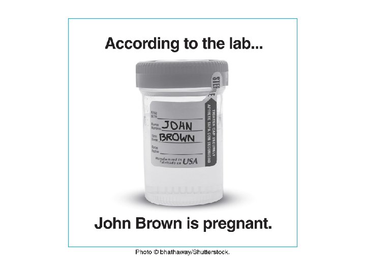
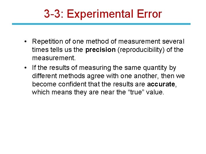
3 -3: Experimental Error • Some laboratory errors are more obvious than others, but there is error associated with every measurement. • There is no way to measure the “true” value of anything. • The best we can do in a chemical analysis is to carefully apply a technique that experience tells us is reliable.

3 -3: Experimental Error • Repetition of one method of measurement several times tells us the precision (reproducibility) of the measurement. • If the results of measuring the same quantity by different methods agree with one another, then we become confident that the results are accurate, which means they are near the “true” value.

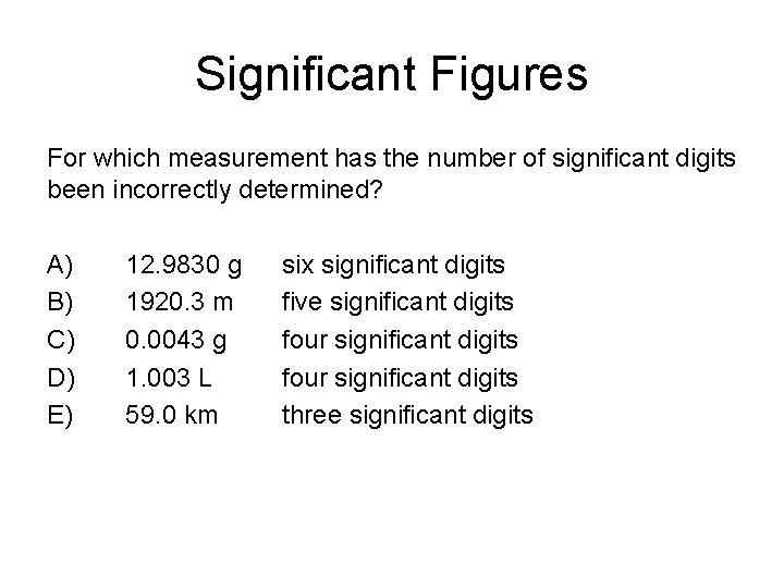
Significant Figures For which measurement has the number of significant digits been incorrectly determined? A) B) C) D) E) 12. 9830 g 1920. 3 m 0. 0043 g 1. 003 L 59. 0 km six significant digits five significant digits four significant digits three significant digits

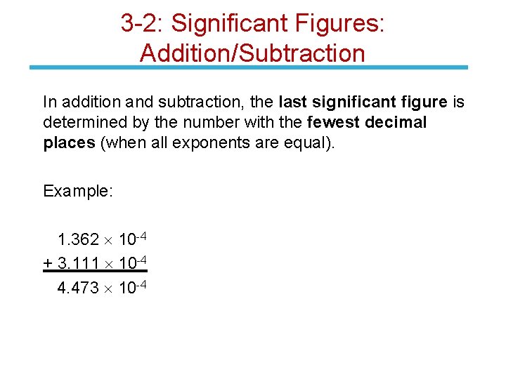
3 -2: Significant Figures: Addition/Subtraction In addition and subtraction, the last significant figure is determined by the number with the fewest decimal places (when all exponents are equal). Example: 1. 362 10 -4 + 3. 111 10 -4 4. 473 10 -4

Calculate the mass of a heterogeneous mixture containing 139. 32 grams sand, 34. 99 grams gravel, and 9. 372 grams salt.

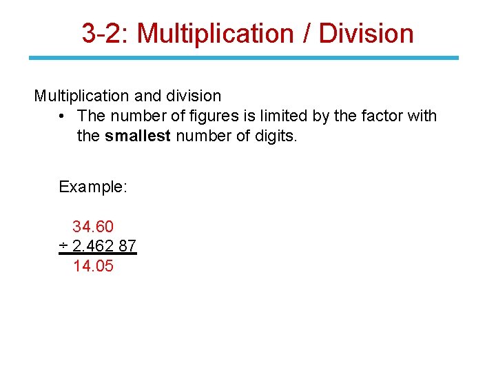
3 -2: Multiplication / Division Multiplication and division • The number of figures is limited by the factor with the smallest number of digits. Example: 34. 60 ÷ 2. 462 87 14. 05

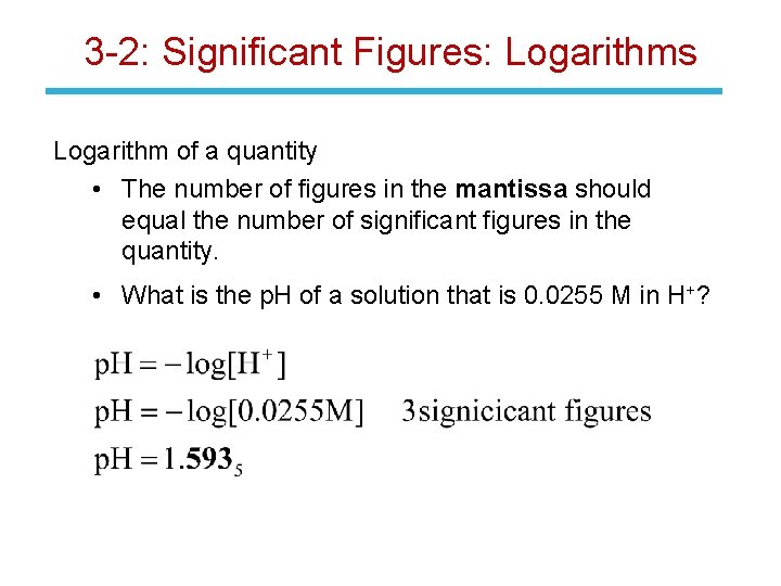
3 -2: Significant Figures: Logarithms Logarithm of a quantity • The number of figures in the mantissa should equal the number of significant figures in the quantity. • What is the p. H of a solution that is 0. 0255 M in H+?

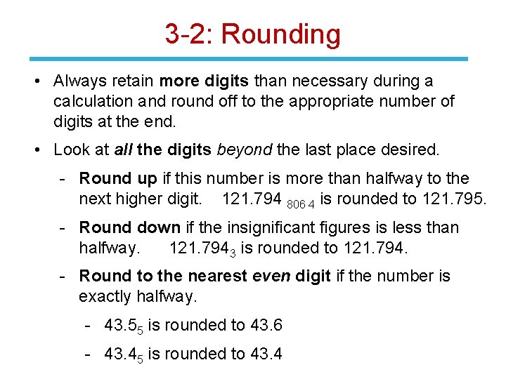
3 -2: Rounding • Always retain more digits than necessary during a calculation and round off to the appropriate number of digits at the end. • Look at all the digits beyond the last place desired. - Round up if this number is more than halfway to the next higher digit. 121. 794 806 4 is rounded to 121. 795. - Round down if the insignificant figures is less than halfway. 121. 7943 is rounded to 121. 794. - Round to the nearest even digit if the number is exactly halfway. - 43. 55 is rounded to 43. 6 - 43. 45 is rounded to 43. 4

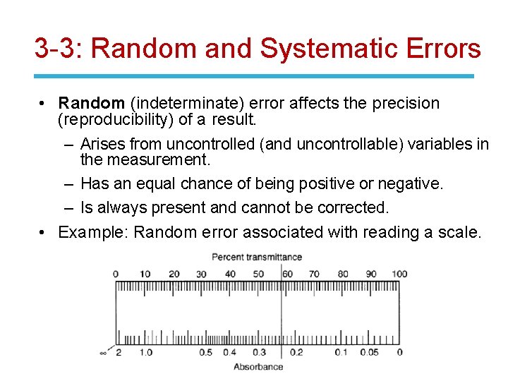
3 -3: Random and Systematic Errors • Random (indeterminate) error affects the precision (reproducibility) of a result. – Arises from uncontrolled (and uncontrollable) variables in the measurement. – Has an equal chance of being positive or negative. – Is always present and cannot be corrected. • Example: Random error associated with reading a scale.

3 -3: Random and Systematic Errors • Systematic (determinate) error affects the accuracy (nearness to the “true” value). – Arises from a flaw in equipment or the design of an experiment. – Reproducible. • Example: An incorrectly standardized p. H meter. You think that the p. H of the buffer used to standardize the meter is 7. 00, but it is really 7. 08. Then all your p. H readings will be 0. 08 p. H unit too low. p. H reading of 5. 60 is actually 5. 68. • With diligence, systematic error can be discovered and eliminated, but some random error is always present. • We strive to eliminate systematic errors in all measurements.

3 -3: Detecting Systematic Error 1. Analyze a known sample, such as a certified reference material. 2. Analyze blank samples containing no analyte being sought. If you observe a nonzero result, your method responds to more than you intend. 3. Use different analytical methods to measure the same quantity. If results do not agree, there is error in one (or more) of the methods. 4. Round robin experiment: Different people in several laboratories analyze identical samples by the same or different methods. 5. Disagreement beyond the estimated random error is systematic error.

3 -3: Uncertainties for Random Errors • We can usually estimate or measure the random error associated with a measurement, such as the length of an object or the temperature of a solution. • Express as the standard deviation, standard deviation of the mean, or a confidence interval, which we discuss in (see Chapter 4). • We assume that systematic error has been detected and corrected.

3 -4: Propagation of Uncertainties from Random Errors • For most experiments, we need to perform arithmetic operations on several numbers, each of which has a random error. • The most likely uncertainty in the result is not the sum of individual errors, because some of them are likely to be positive and some negative. • We expect some cancellation of errors.

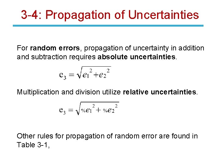
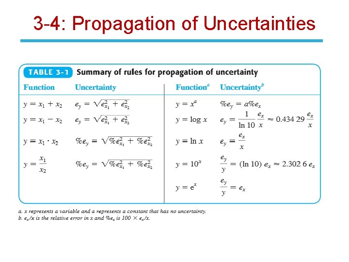
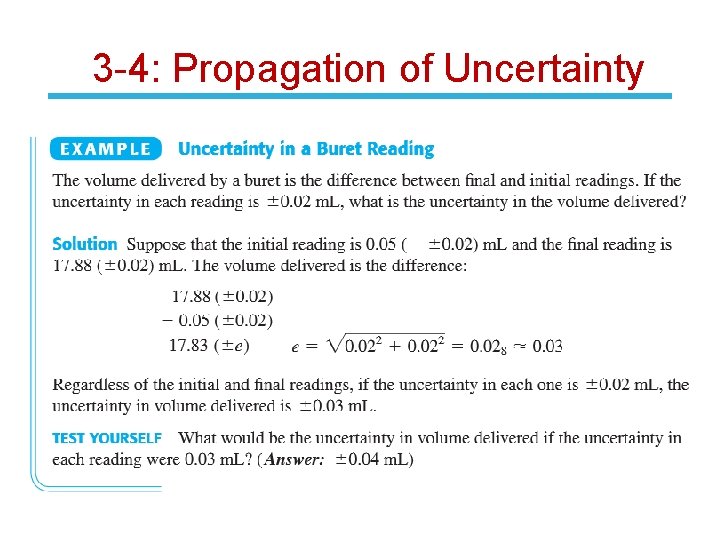
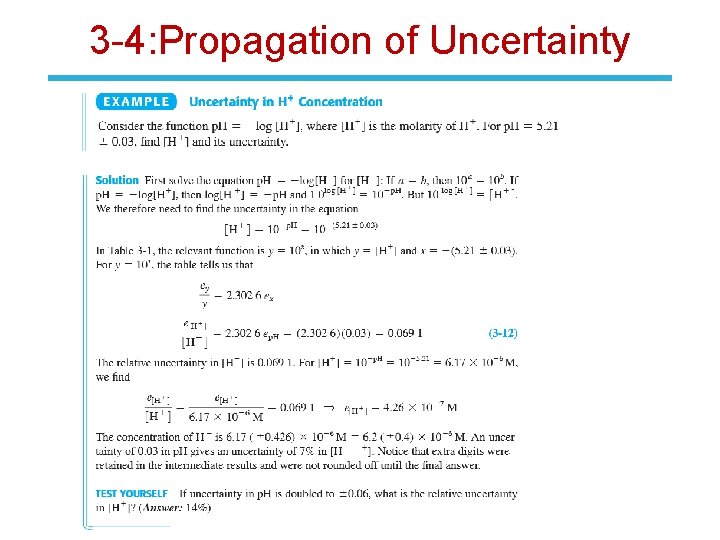
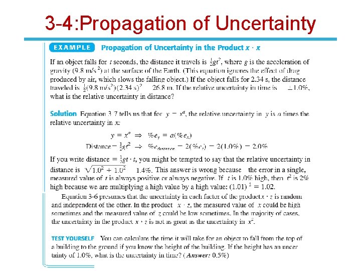
3 -4: Propagation of Uncertainties For random errors, propagation of uncertainty in addition and subtraction requires absolute uncertainties. Multiplication and division utilize relative uncertainties. Other rules for propagation of random error are found in Table 3 -1,

3 -4: Propagation of Uncertainties

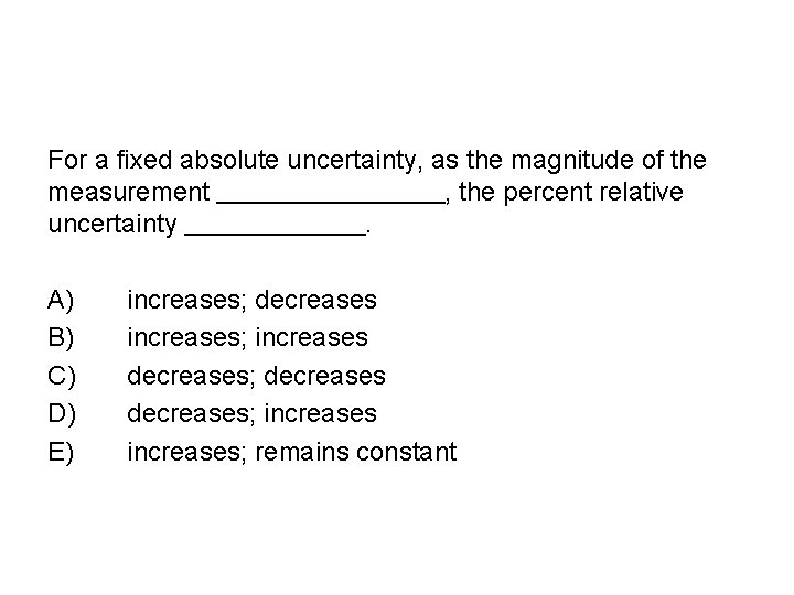
For a fixed absolute uncertainty, as the magnitude of the measurement , the percent relative uncertainty. A) B) C) D) E) increases; decreases increases; increases decreases; increases; remains constant

3 -4: Propagation of Uncertainty

3 -4: Propagation of Uncertainty

3 -4: Propagation of Uncertainty

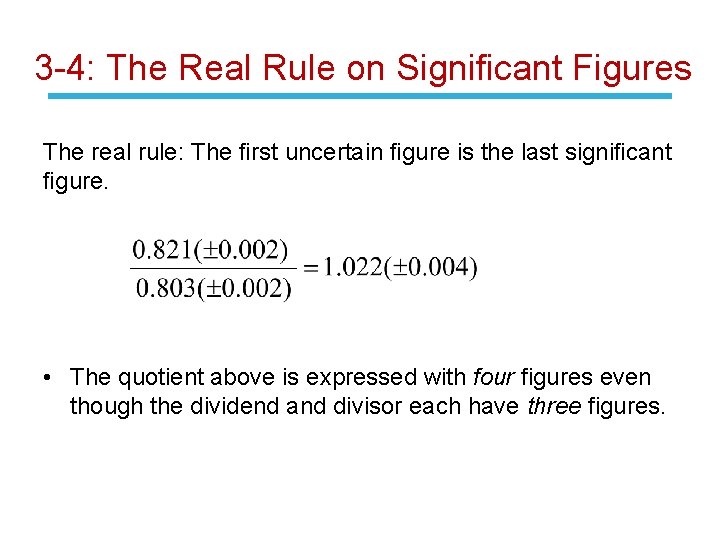
3 -4: The Real Rule on Significant Figures The real rule: The first uncertain figure is the last significant figure. • The quotient above is expressed with four figures even though the dividend and divisor each have three figures.

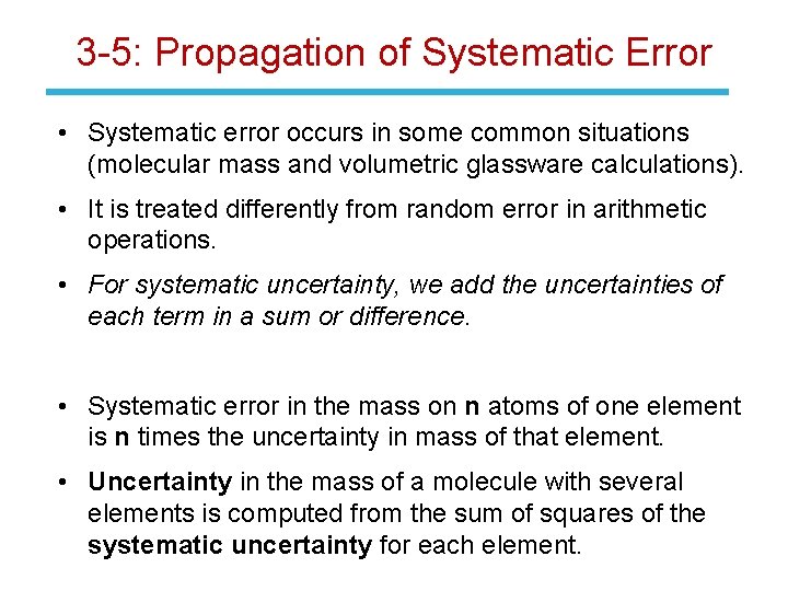
3 -5: Propagation of Systematic Error • Systematic error occurs in some common situations (molecular mass and volumetric glassware calculations). • It is treated differently from random error in arithmetic operations. • For systematic uncertainty, we add the uncertainties of each term in a sum or difference. • Systematic error in the mass on n atoms of one element is n times the uncertainty in mass of that element. • Uncertainty in the mass of a molecule with several elements is computed from the sum of squares of the systematic uncertainty for each element.

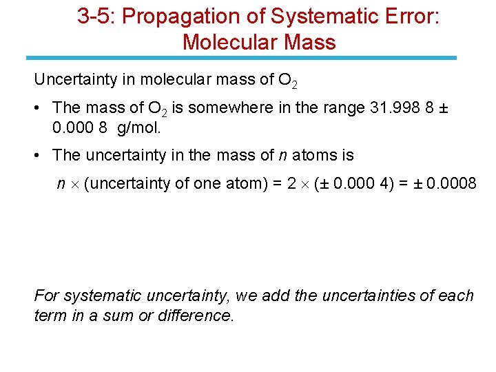
3 -5: Propagation of Systematic Error: Molecular Mass Uncertainty in molecular mass of O 2 • The mass of O 2 is somewhere in the range 31. 998 8 ± 0. 000 8 g/mol. • The uncertainty in the mass of n atoms is n (uncertainty of one atom) = 2 (± 0. 000 4) = ± 0. 0008 For systematic uncertainty, we add the uncertainties of each term in a sum or difference.

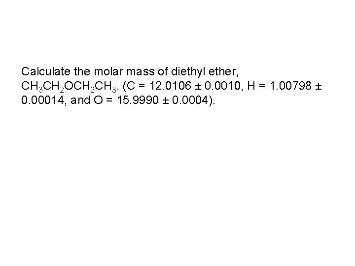
Calculate the molar mass of diethyl ether, CH 3 CH 2 OCH 2 CH 3. (C = 12. 0106 ± 0. 0010, H = 1. 00798 ± 0. 00014, and O = 15. 9990 ± 0. 0004).

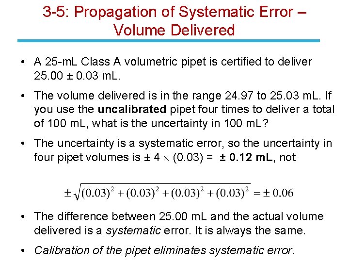
3 -5: Propagation of Systematic Error – Volume Delivered • A 25 -m. L Class A volumetric pipet is certified to deliver 25. 00 ± 0. 03 m. L. • The volume delivered is in the range 24. 97 to 25. 03 m. L. If you use the uncalibrated pipet four times to deliver a total of 100 m. L, what is the uncertainty in 100 m. L? • The uncertainty is a systematic error, so the uncertainty in four pipet volumes is ± 4 (0. 03) = ± 0. 12 m. L, not • The difference between 25. 00 m. L and the actual volume delivered is a systematic error. It is always the same. • Calibration of the pipet eliminates systematic error.

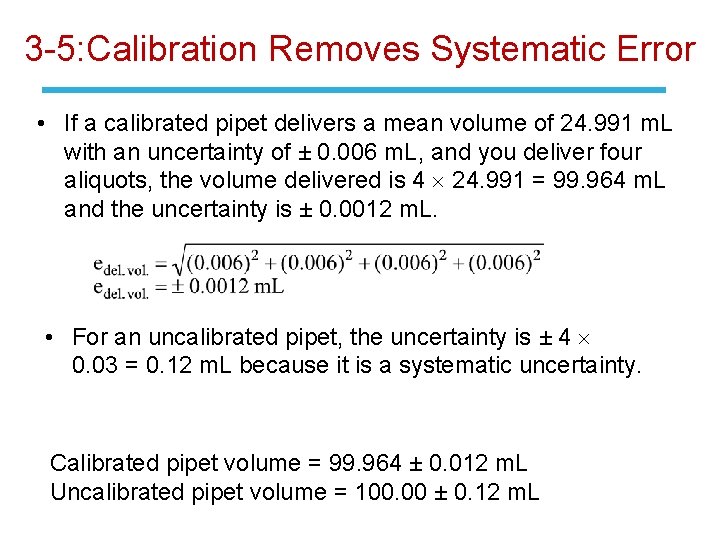
3 -5: Calibration Removes Systematic Error • If a calibrated pipet delivers a mean volume of 24. 991 m. L with an uncertainty of ± 0. 006 m. L, and you deliver four aliquots, the volume delivered is 4 24. 991 = 99. 964 m. L and the uncertainty is ± 0. 0012 m. L. • For an uncalibrated pipet, the uncertainty is ± 4 0. 03 = 0. 12 m. L because it is a systematic uncertainty. Calibrated pipet volume = 99. 964 ± 0. 012 m. L Uncalibrated pipet volume = 100. 00 ± 0. 12 m. L

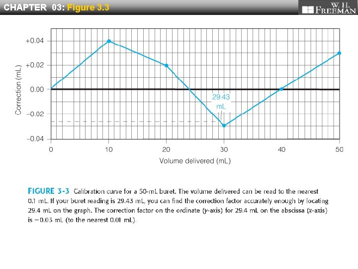
CHAPTER 03: Figure 3. 3

END