Chapter 3 Descriptive Statistics Numerical Measures n n

Chapter 3 Descriptive Statistics: Numerical Measures n n Measures of Location Measures of Variability

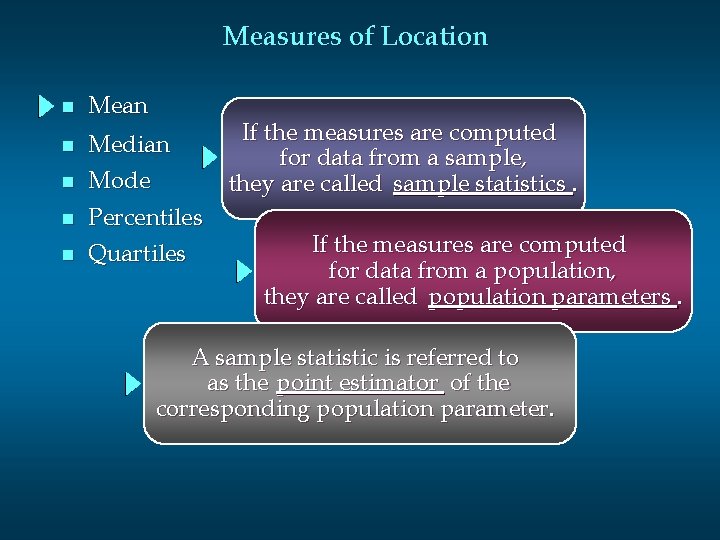
Measures of Location n Mean n Median Mode n n n Percentiles Quartiles If the measures are computed for data from a sample, they are called sample statistics. If the measures are computed for data from a population, they are called population parameters. A sample statistic is referred to as the point estimator of the corresponding population parameter.

Mean n n The mean of a data set is the average of all the data values. The sample mean is the point estimator of the population mean m.

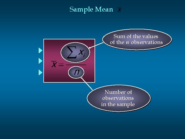
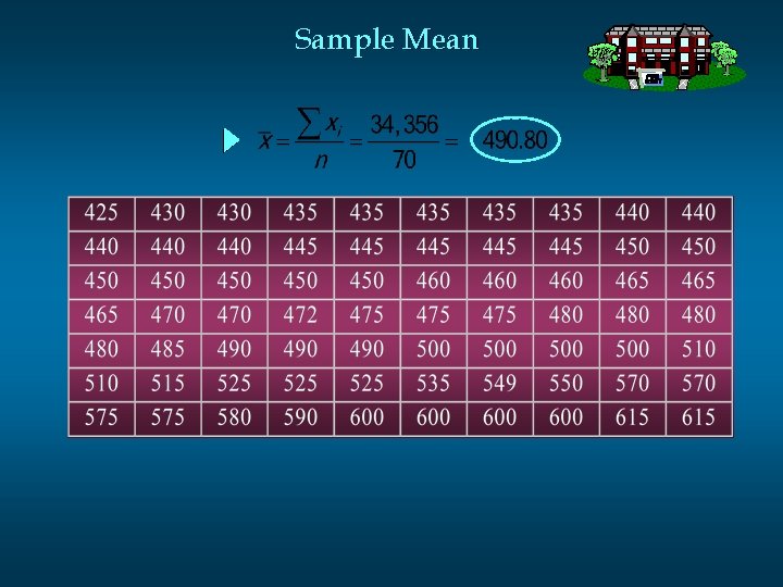
Sample Mean Sum of the values of the n observations Number of observations in the sample

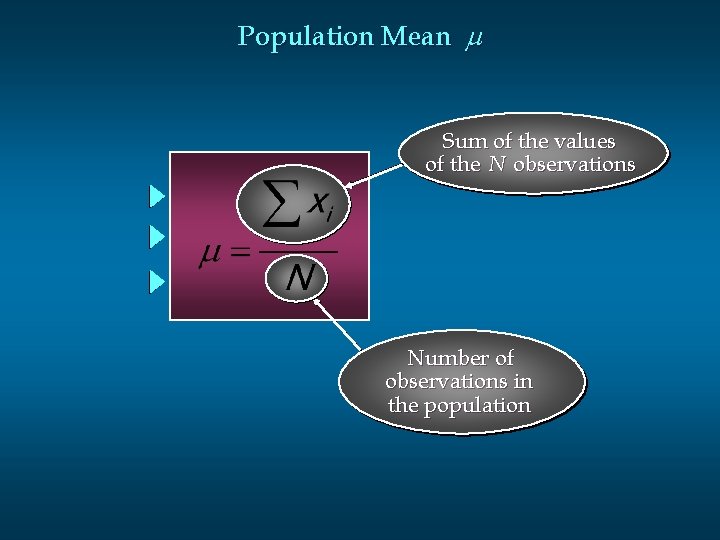
Population Mean m Sum of the values of the N observations Number of observations in the population

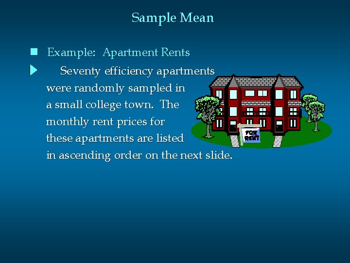
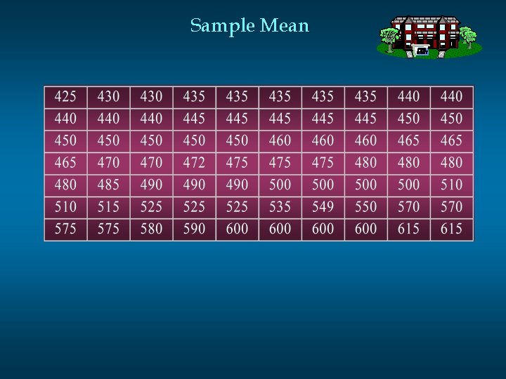
Sample Mean n Example: Apartment Rents Seventy efficiency apartments were randomly sampled in a small college town. The monthly rent prices for these apartments are listed in ascending order on the next slide.

Sample Mean

Sample Mean

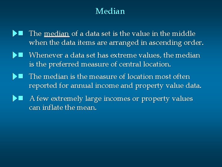
Median n The median of a data set is the value in the middle when the data items are arranged in ascending order. n Whenever a data set has extreme values, the median is the preferred measure of central location. n The median is the measure of location most often reported for annual income and property value data. n A few extremely large incomes or property values can inflate the mean.

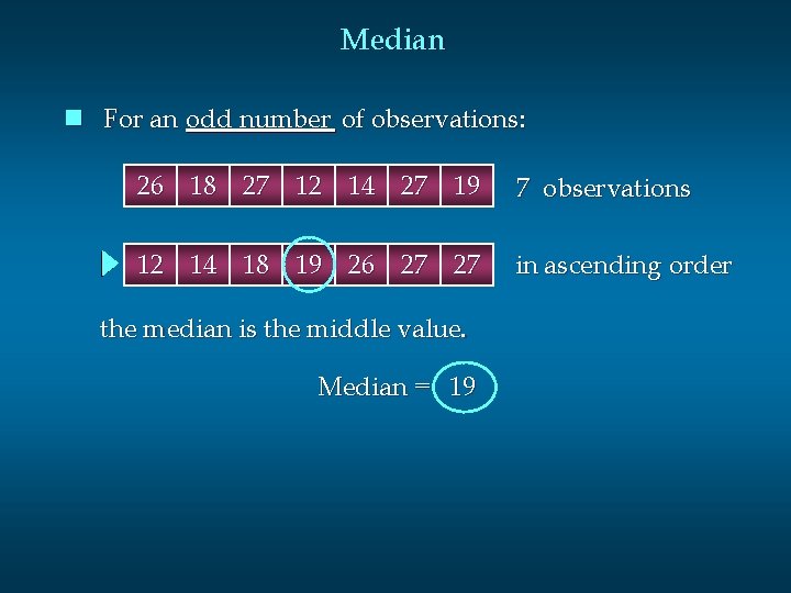
Median n For an odd number of observations: 26 18 27 12 14 27 19 7 observations 12 14 18 19 26 27 27 in ascending order the median is the middle value. Median = 19

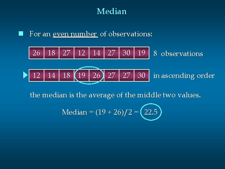
Median n For an even number of observations: 26 18 27 12 14 27 30 19 8 observations 12 14 18 19 26 27 27 30 in ascending order the median is the average of the middle two values. Median = (19 + 26)/2 = 22. 5

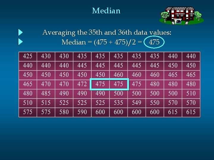
Median Averaging the 35 th and 36 th data values: Median = (475 + 475)/2 = 475

Mode n The mode of a data set is the value that occurs with greatest frequency. n The greatest frequency can occur at two or more different values. n If the data have exactly two modes, the data are bimodal. n If the data have more than two modes, the data are multimodal.

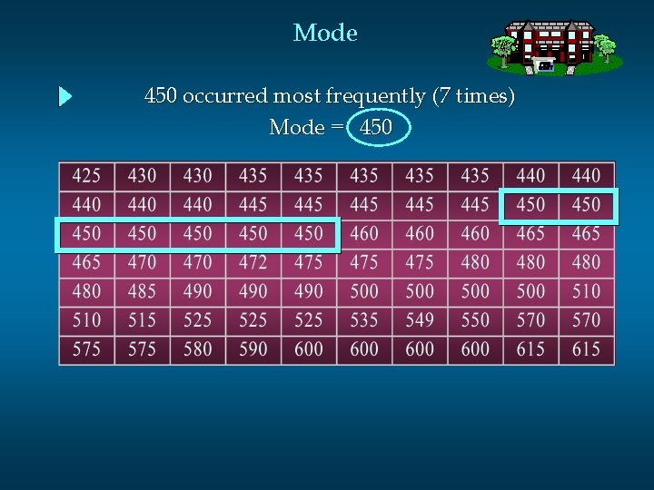
Mode 450 occurred most frequently (7 times) Mode = 450

Percentiles n A percentile provides information about how the data are spread over the interval from the smallest value to the largest value. n Admission test scores for colleges and universities are frequently reported in terms of percentiles.

Percentiles n The p th percentile of a data set is a value such that at least p percent of the items take on this value or less and at least (100 - p ) percent of the items take on this value or more.

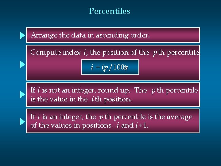
Percentiles Arrange the data in ascending order. Compute index i , the position of the p th percentile. i = (p /100)n If i is not an integer, round up. The p th percentile is the value in the i th position. If i is an integer, the p th percentile is the average of the values in positions i and i +1.

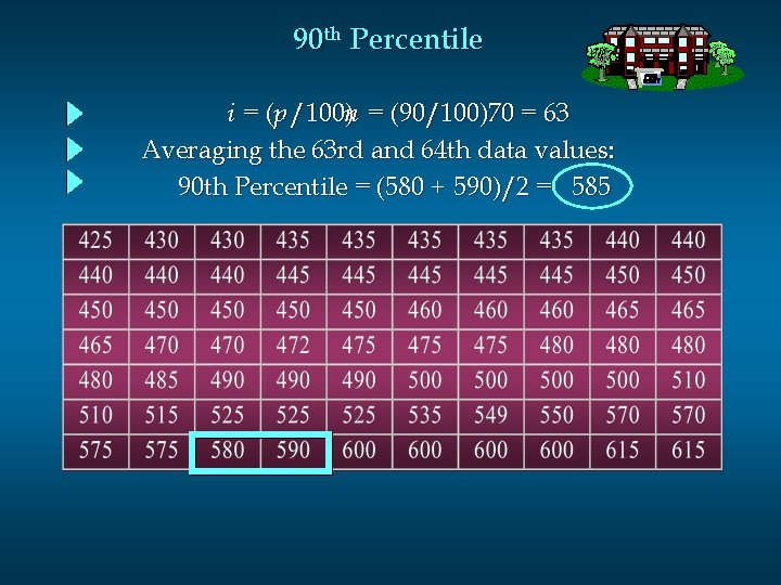
90 th Percentile i = (p /100)n = (90/100)70 = 63 Averaging the 63 rd and 64 th data values: 90 th Percentile = (580 + 590)/2 = 585

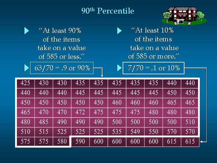
90 th Percentile “At least 90% of the items take on a value of 585 or less. ” “At least 10% of the items take on a value of 585 or more. ” 63/70 =. 9 or 90% 7/70 =. 1 or 10%

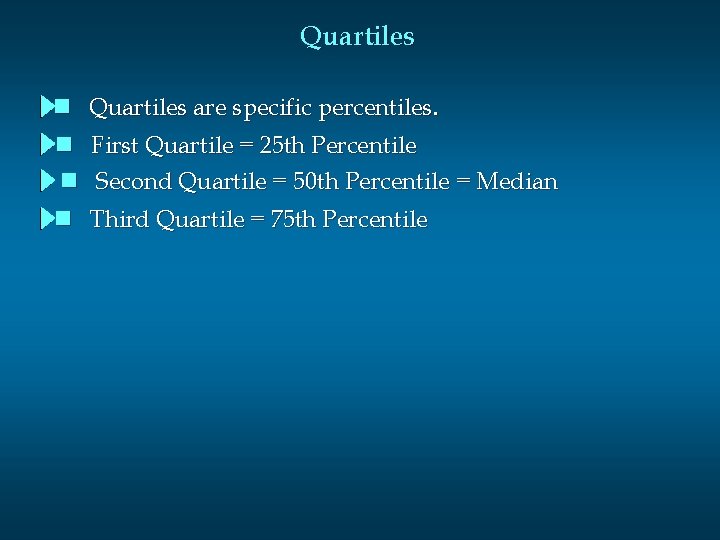
Quartiles n n n Quartiles are specific percentiles. First Quartile = 25 th Percentile Second Quartile = 50 th Percentile = Median n Third Quartile = 75 th Percentile

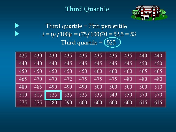
Third Quartile Third quartile = 75 th percentile i = (p /100)n = (75/100)70 = 52. 5 = 53 Third quartile = 525

Measures of Variability n It is often desirable to consider measures of variability (dispersion), as well as measures of location. n For example, in choosing supplier A or supplier B we might consider not only the average delivery time for each, but also the variability in delivery time for each.

Measures of Variability n Range n Interquartile Range n Variance n Standard Deviation n Coefficient of Variation

Range n The range of a data set is the difference between the largest and smallest data values. n It is the simplest measure of variability. n It is very sensitive to the smallest and largest data values.

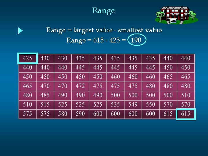
Range = largest value - smallest value Range = 615 - 425 = 190

Interquartile Range n The interquartile range of a data set is the difference between the third quartile and the first quartile. n It is the range for the middle 50% of the data. n It overcomes the sensitivity to extreme data values.

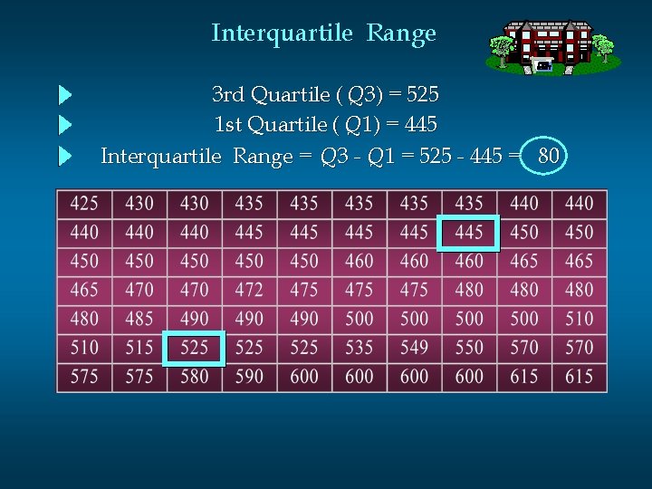
Interquartile Range 3 rd Quartile ( Q 3) = 525 1 st Quartile ( Q 1) = 445 Interquartile Range = Q 3 - Q 1 = 525 - 445 = 80

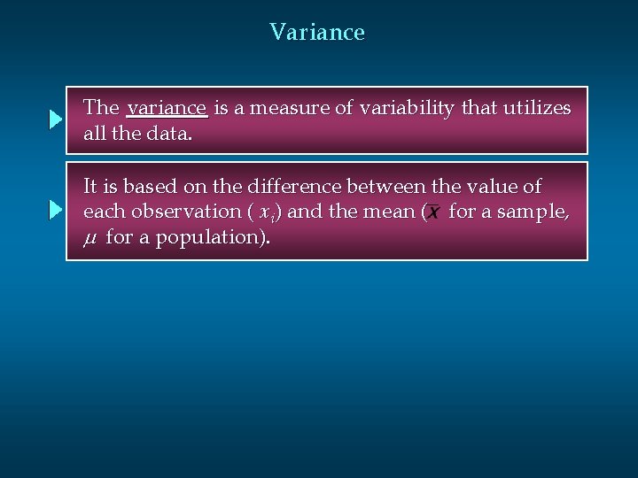
Variance The variance is a measure of variability that utilizes all the data. It is based on the difference between the value of each observation ( xi ) and the mean ( for a sample, m for a population).

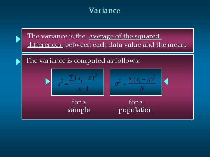
Variance The variance is the average of the squared differences between each data value and the mean. The variance is computed as follows: for a sample for a population

Standard Deviation The standard deviation of a data set is the positive square root of the variance. It is measured in the same units as the data , making it more easily interpreted than the variance.

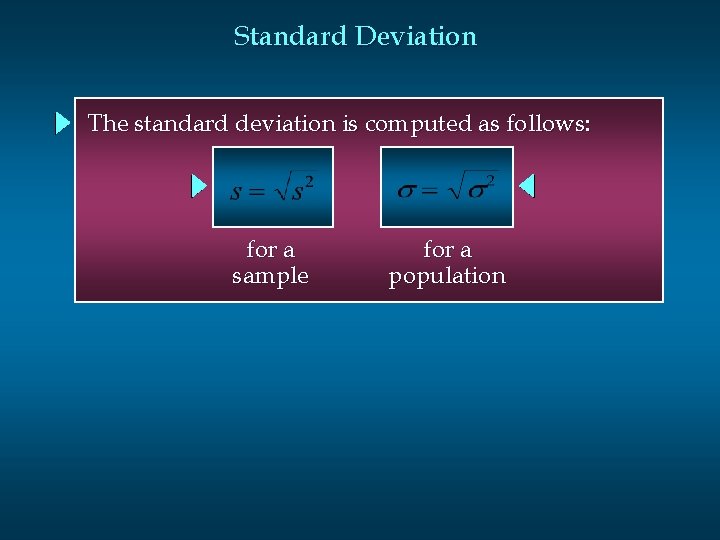
Standard Deviation The standard deviation is computed as follows: for a sample for a population

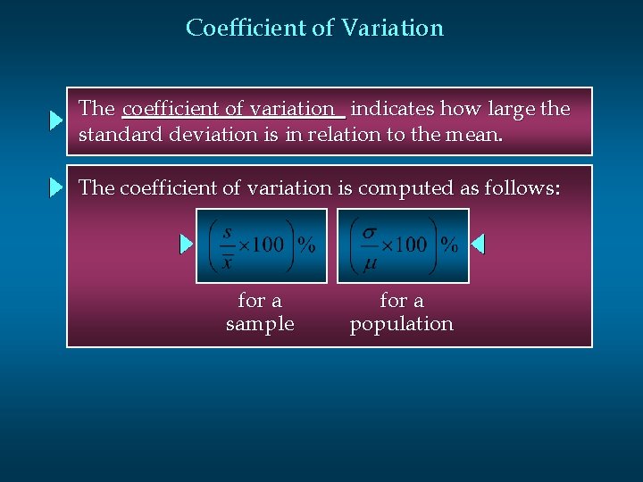
Coefficient of Variation The coefficient of variation indicates how large the standard deviation is in relation to the mean. The coefficient of variation is computed as follows: for a sample for a population

Descriptive Statistics: Numerical Measures n Measures of Distribution Shape, Relative Location, and Detecting Outliers

Measures of Distribution Shape, Relative Location, and Detecting Outliers n n n Distribution Shape z-Scores Detecting Outliers

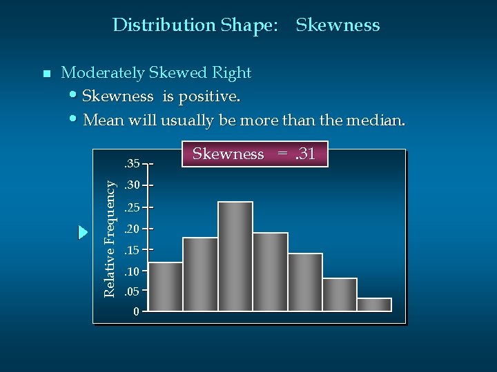
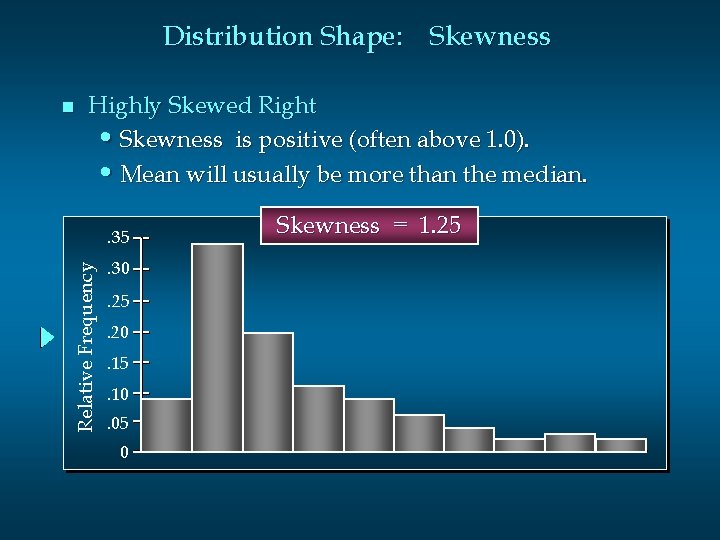
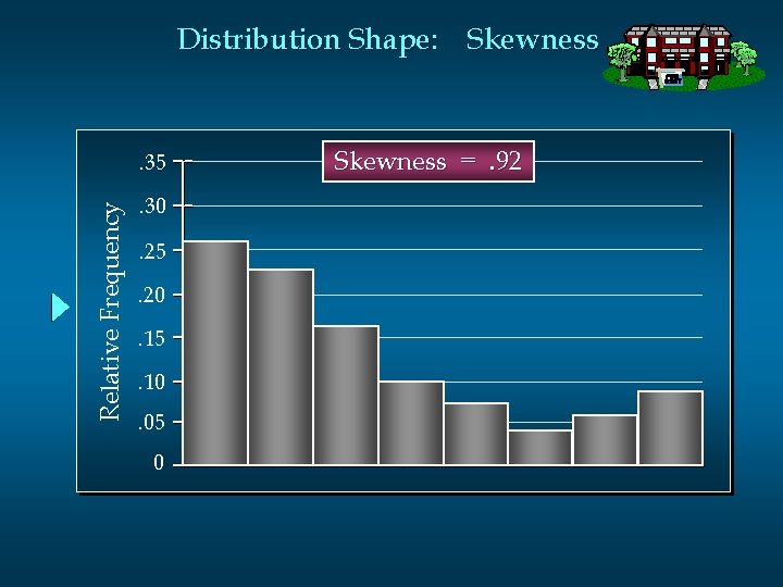
Distribution Shape: Skewness n An important measure of the shape of a distribution is called skewness. n The formula for computing skewness for a data set is somewhat complex. n Skewness can be easily computed using statistical software.

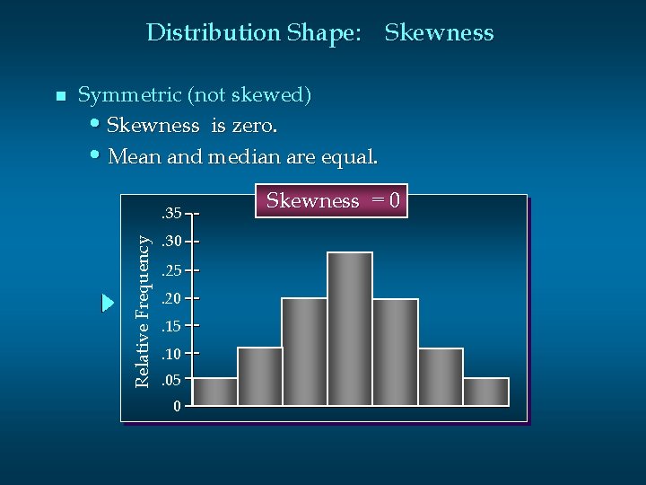
Distribution Shape: Skewness Symmetric (not skewed) • Skewness is zero. • Mean and median are equal. . 35 Relative Frequency n . 30. 25. 20. 15. 10. 05 0 Skewness = 0

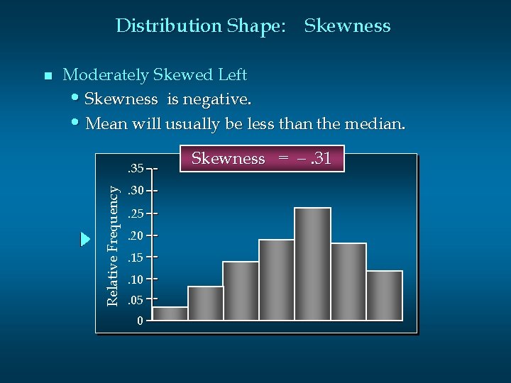
Distribution Shape: Skewness Moderately Skewed Left • Skewness is negative. • Mean will usually be less than the median. . 35 Relative Frequency n . 30. 25. 20. 15. 10. 05 0 Skewness = -. 31

Distribution Shape: Skewness Moderately Skewed Right • Skewness is positive. • Mean will usually be more than the median. . 35 Relative Frequency n . 30. 25. 20. 15. 10. 05 0 Skewness =. 31

Distribution Shape: Skewness n Highly Skewed Right • Skewness is positive (often above 1. 0). • Mean will usually be more than the median. Relative Frequency . 35. 30. 25. 20. 15. 10. 05 0 Skewness = 1. 25

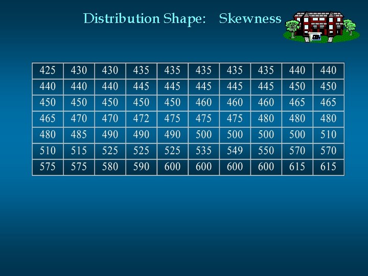
Distribution Shape: Skewness n Example: Apartment Rents Seventy efficiency apartments were randomly sampled in a small college town. The monthly rent prices for these apartments are listed in ascending order on the next slide.

Distribution Shape: Skewness

Distribution Shape: Skewness Relative Frequency . 35. 30. 25. 20. 15. 10. 05 0 Skewness =. 92

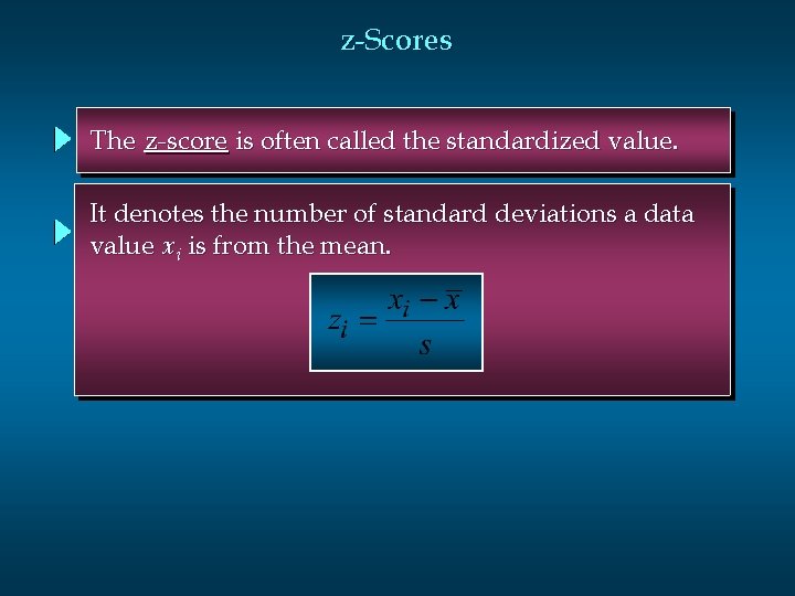
z-Scores The z-score is often called the standardized value. It denotes the number of standard deviations a data value xi is from the mean.

z-Scores n An observation’s z-score is a measure of the relative location of the observation in a data set. n A data value less than the sample mean will have a z-score less than zero. n A data value greater than the sample mean will have a z-score greater than zero. n A data value equal to the sample mean will have a z-score of zero.

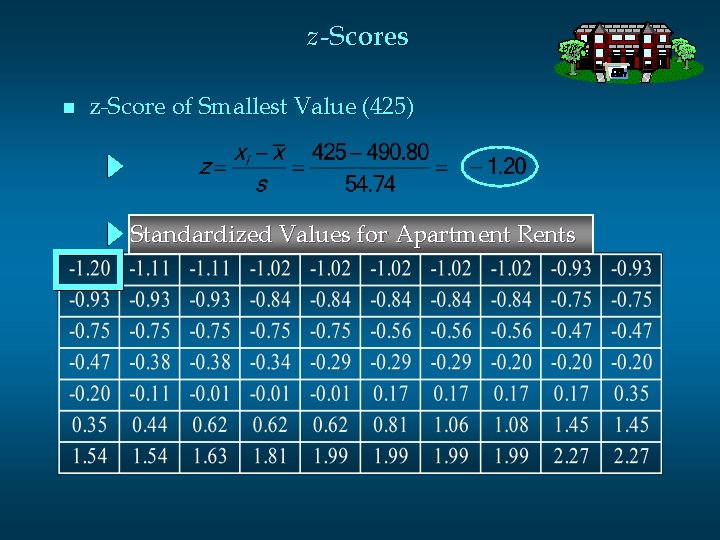
z -Scores n z-Score of Smallest Value (425) Standardized Values for Apartment Rents

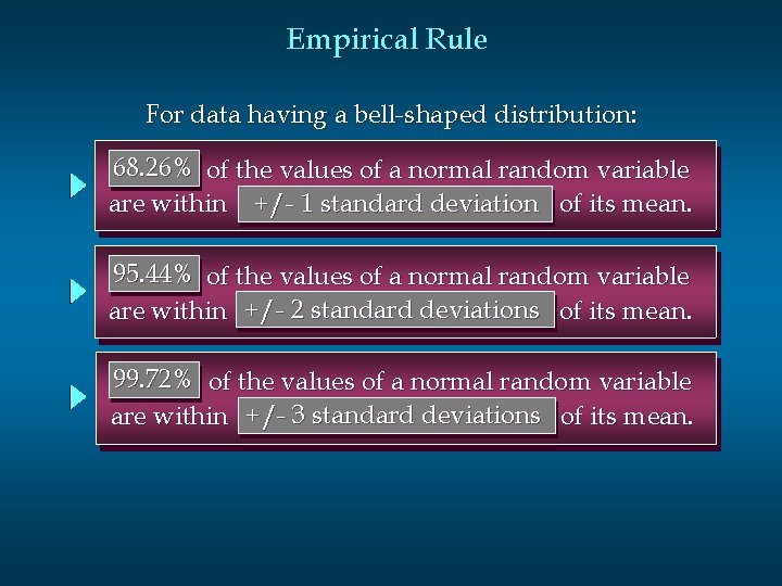
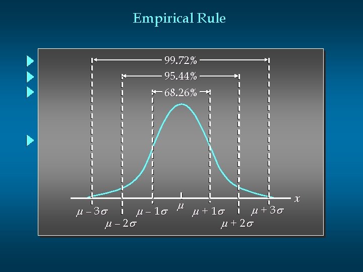
Empirical Rule For data having a bell-shaped distribution: 68. 26% of the values of a normal random variable are within +/- 1 standard deviation of its mean. 95. 44% of the values of a normal random variable are within +/- 2 standard deviations of its mean. 99. 72% of the values of a normal random variable are within +/- 3 standard deviations of its mean.

Empirical Rule 99. 72% 95. 44% 68. 26% m m + 3 s m – 1 s m + 1 s m – 2 s m + 2 s x

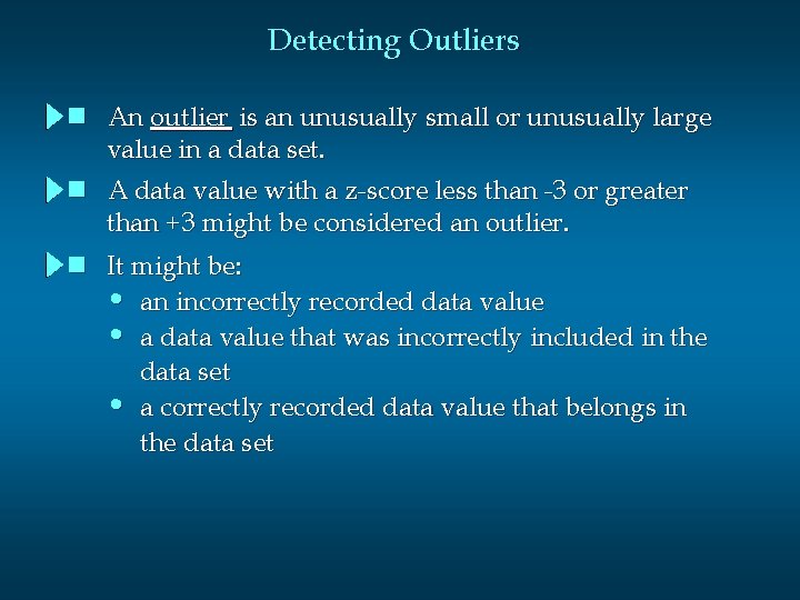
Detecting Outliers n An outlier is an unusually small or unusually large value in a data set. n A data value with a z-score less than -3 or greater than +3 might be considered an outlier. n It might be: • an incorrectly recorded data value • a data value that was incorrectly included in the data set • a correctly recorded data value that belongs in the data set

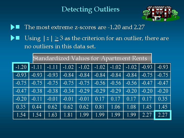
Detecting Outliers n The most extreme z-scores are -1. 20 and 2. 27 n Using | z | > 3 as the criterion for an outlier, there are no outliers in this data set. Standardized Values for Apartment Rents