Chapter 3 Descriptive Statistics BUSINESS STATISTICS 4 E
Chapter 3: Descriptive Statistics BUSINESS STATISTICS, 4 E, BY KEN BLACK. © 2003 JOHN WILEY & SONS. 3 -1
Learning Objectives 1. Distinguish between measures of central tendency, measures of variability, measures of shape, and measures of association. 2. Understand the meanings of mean, median, mode, quartile, percentile, and range. 3. Compute mean, median, mode, percentile, quartile, range, variance, standard deviation, and mean absolute deviation on ungrouped data. 4. Differentiate between sample and population variance and standard deviation. BUSINESS STATISTICS, 4 E, BY KEN BLACK. © 2003 JOHN WILEY & SONS. 3 -2
Learning Objectives -- Continued 5. Understand the meaning of standard deviation as it is applied by using the empirical rule and Chebyshev’s theorem. 6. Compute the mean, median, standard deviation, and variance on grouped data. 7. Understand box and whisker plots, skewness, and kurtosis. 8. Compute a coefficient of correlation and interpret it. BUSINESS STATISTICS, 4 E, BY KEN BLACK. © 2003 JOHN WILEY & SONS. 3 -3
Measures of Central Tendency: Ungrouped Data Measures of central tendency yield information about “particular places or locations in a group of numbers. ” Common Measures of Location ◦ ◦ ◦ Mode Median Mean Percentiles Quartiles BUSINESS STATISTICS, 4 E, BY KEN BLACK. © 2003 JOHN WILEY & SONS. 3 -4
Mode The most frequently occurring value in a data set Applicable to all levels of data measurement (nominal, ordinal, interval, and ratio) Bimodal -- Data sets that have two modes Multimodal -- Data sets that contain more than two modes BUSINESS STATISTICS, 4 E, BY KEN BLACK. © 2003 JOHN WILEY & SONS. 3 -5
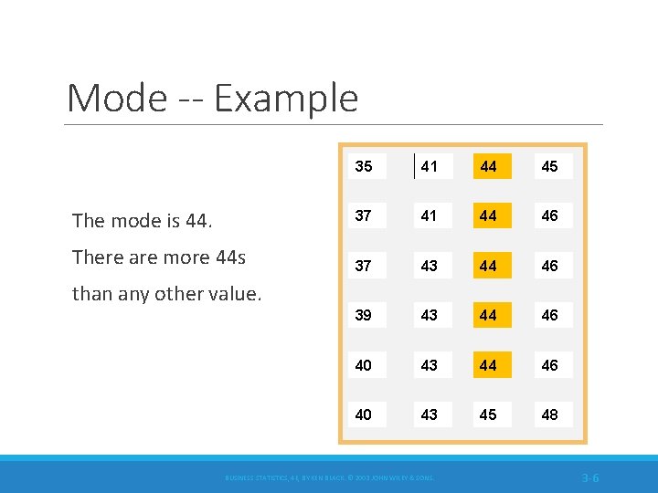
Mode -- Example The mode is 44. There are more 44 s 35 41 44 45 37 41 44 46 37 43 44 46 39 43 44 46 40 43 45 48 than any other value. BUSINESS STATISTICS, 4 E, BY KEN BLACK. © 2003 JOHN WILEY & SONS. 3 -6
Median • Middle value in an ordered array of numbers. • Applicable for ordinal, interval, and ratio data • Not applicable for nominal data • Unaffected by extremely large and extremely small values. BUSINESS STATISTICS, 4 E, BY KEN BLACK. © 2003 JOHN WILEY & SONS. 3 -7
Median: Computational Procedure First Procedure ◦ Arrange the observations in an ordered array. ◦ If there is an odd number of terms, the median is the middle term of the ordered array. ◦ If there is an even number of terms, the median is the average of the middle two terms. Second Procedure ◦ The median’s position in an ordered array is given by (n+1)/2. BUSINESS STATISTICS, 4 E, BY KEN BLACK. © 2003 JOHN WILEY & SONS. 3 -8

Median: Example with an Odd Number of Terms Ordered Array 3 4 5 7 8 9 11 14 15 16 16 17 19 19 20 21 22 There are 17 terms in the ordered array. Position of median = (n+1)/2 = (17+1)/2 = 9 The median is the 9 th term, 15. If the 22 is replaced by 100, the median is 15. If the 3 is replaced by -103, the median is 15. BUSINESS STATISTICS, 4 E, BY KEN BLACK. © 2003 JOHN WILEY & SONS. 3 -9

Median: Example with an Even Number of Terms Ordered Array 3 4 5 7 8 9 11 14 15 16 16 17 19 19 20 21 • There are 16 terms in the ordered array. • Position of median = (n+1)/2 = (16+1)/2 = 8. 5 • The median is between the 8 th and 9 th terms, 14. 5. • If the 21 is replaced by 100, the median is 14. 5. • If the 3 is replaced by -88, the median is 14. 5. BUSINESS STATISTICS, 4 E, BY KEN BLACK. © 2003 JOHN WILEY & SONS. 3 -10
Arithmetic Mean Commonly called ‘the mean’ is the average of a group of numbers Applicable for interval and ratio data Not applicable for nominal or ordinal data Affected by each value in the data set, including extreme values Computed by summing all values in the data set and dividing the sum by the number of values in the data set BUSINESS STATISTICS, 4 E, BY KEN BLACK. © 2003 JOHN WILEY & SONS. 3 -11
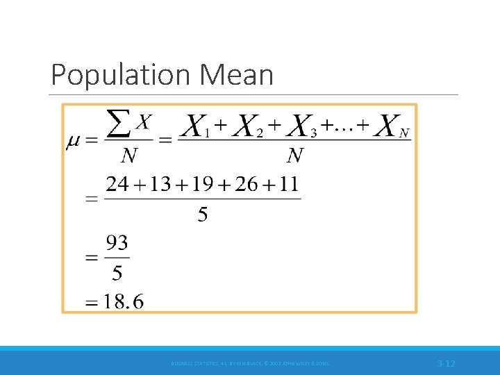
Population Mean BUSINESS STATISTICS, 4 E, BY KEN BLACK. © 2003 JOHN WILEY & SONS. 3 -12
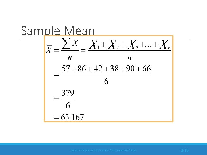
Sample Mean BUSINESS STATISTICS, 4 E, BY KEN BLACK. © 2003 JOHN WILEY & SONS. 3 -13
Percentiles Measures of central tendency that divide a group of data into 100 parts At least n% of the data lie below the nth percentile, and at most (100 - n)% of the data lie above the nth percentile Example: 90 th percentile indicates that at least 90% of the data lie below it, and at most 10% of the data lie above it The median and the 50 th percentile have the same value. Applicable for ordinal, interval, and ratio data Not applicable for nominal data BUSINESS STATISTICS, 4 E, BY KEN BLACK. © 2003 JOHN WILEY & SONS. 3 -14

Percentiles: Computational Procedure Organize the data into an ascending ordered array. Calculate the percentile location: Determine the percentile’s location and its value. If i is a whole number, the percentile is the average of the values at the i and (i+1) positions. If i is not a whole number, the percentile is at the (i+1) position in the ordered array. BUSINESS STATISTICS, 4 E, BY KEN BLACK. © 2003 JOHN WILEY & SONS. 3 -15
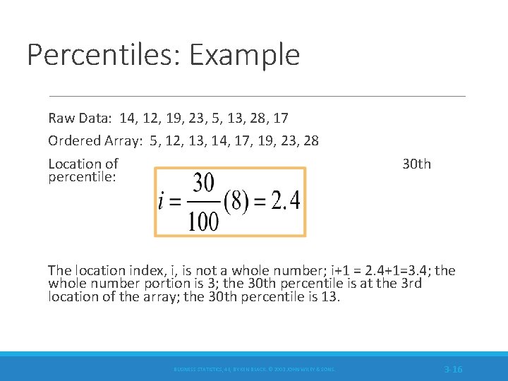
Percentiles: Example Raw Data: 14, 12, 19, 23, 5, 13, 28, 17 Ordered Array: 5, 12, 13, 14, 17, 19, 23, 28 Location of percentile: 30 th The location index, i, is not a whole number; i+1 = 2. 4+1=3. 4; the whole number portion is 3; the 30 th percentile is at the 3 rd location of the array; the 30 th percentile is 13. BUSINESS STATISTICS, 4 E, BY KEN BLACK. © 2003 JOHN WILEY & SONS. 3 -16
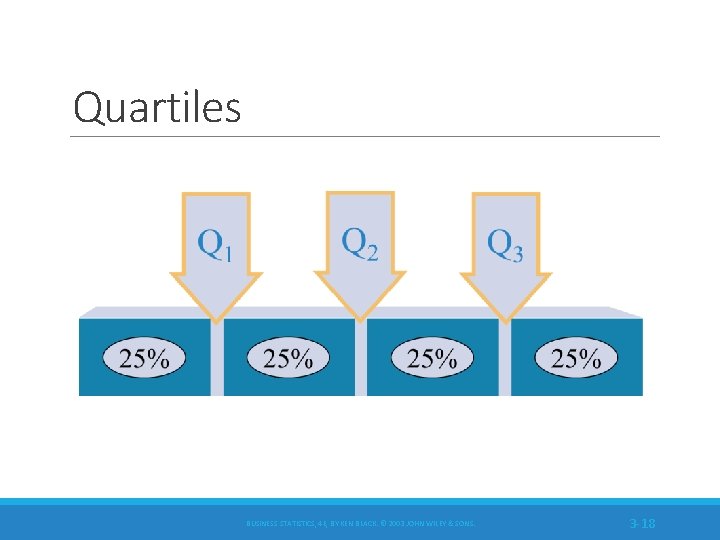
Quartiles Measures of central tendency that divide a group of data into four subgroups Q 1: 25% of the data set is below the first quartile Q 2: 50% of the data set is below the second quartile Q 3: 75% of the data set is below the third quartile Q 1 is equal to the 25 th percentile Q 2 is located at 50 th percentile and equals the median Q 3 is equal to the 75 th percentile Quartile values are not necessarily members of the data set BUSINESS STATISTICS, 4 E, BY KEN BLACK. © 2003 JOHN WILEY & SONS. 3 -17
Quartiles BUSINESS STATISTICS, 4 E, BY KEN BLACK. © 2003 JOHN WILEY & SONS. 3 -18
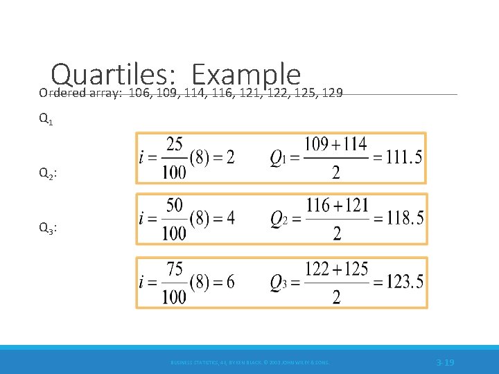
Quartiles: Example Ordered array: 106, 109, 114, 116, 121, 122, 125, 129 Q 1 Q 2 : Q 3 : BUSINESS STATISTICS, 4 E, BY KEN BLACK. © 2003 JOHN WILEY & SONS. 3 -19
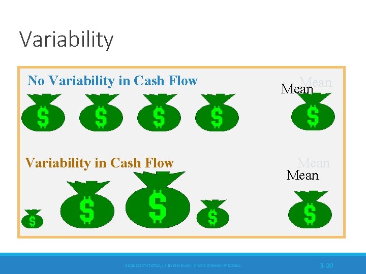
Variability No Variability in Cash Flow BUSINESS STATISTICS, 4 E, BY KEN BLACK. © 2003 JOHN WILEY & SONS. Mean 3 -20
Variability No Variability BUSINESS STATISTICS, 4 E, BY KEN BLACK. © 2003 JOHN WILEY & SONS. 3 -21
Measures of Variability: Ungrouped Data Measures of variability describe the spread or the dispersion of a set of data. Common Measures of Variability ◦ ◦ ◦ ◦ Range Interquartile Range Mean Absolute Deviation Variance Standard Deviation Z scores Coefficient of Variation BUSINESS STATISTICS, 4 E, BY KEN BLACK. © 2003 JOHN WILEY & SONS. 3 -22
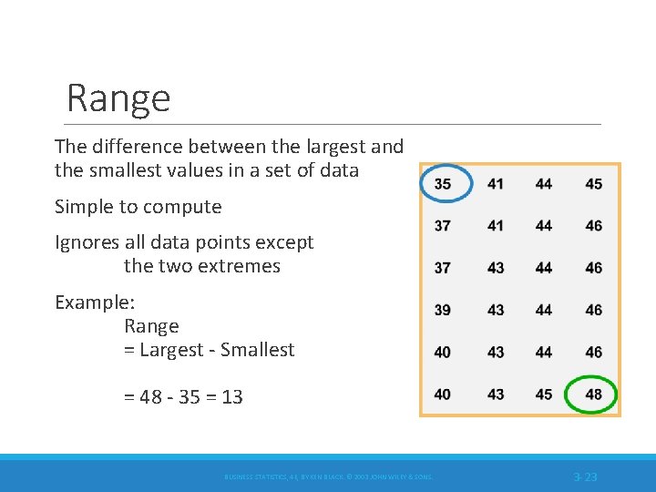
Range The difference between the largest and the smallest values in a set of data Simple to compute Ignores all data points except the two extremes Example: Range = Largest - Smallest = 48 - 35 = 13 BUSINESS STATISTICS, 4 E, BY KEN BLACK. © 2003 JOHN WILEY & SONS. 3 -23

Interquartile Range of values between the first and third quartiles Range of the “middle half” Less influenced by extremes BUSINESS STATISTICS, 4 E, BY KEN BLACK. © 2003 JOHN WILEY & SONS. 3 -24
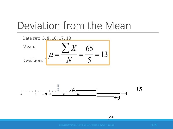
Deviation from the Mean Data set: 5, 9, 16, 17, 18 Mean: Deviations from the mean: -8, -4, 3, 4, 5 -8 -4 +3 BUSINESS STATISTICS, 4 E, BY KEN BLACK. © 2003 JOHN WILEY & SONS. +4 +5 3 -25
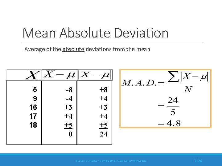
Mean Absolute Deviation Average of the absolute deviations from the mean 5 9 16 17 18 -8 -4 +3 +4 +5 0 +8 +4 +3 +4 +5 24 BUSINESS STATISTICS, 4 E, BY KEN BLACK. © 2003 JOHN WILEY & SONS. 3 -26
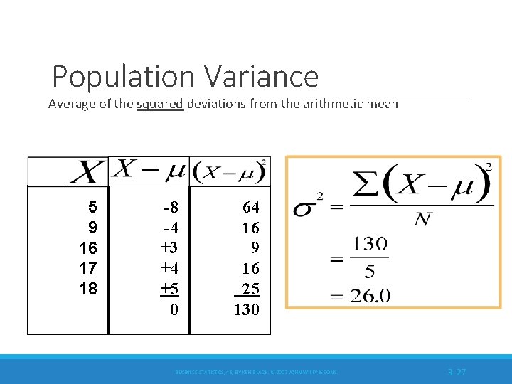
Population Variance Average of the squared deviations from the arithmetic mean 5 9 16 17 18 -8 -4 +3 +4 +5 0 64 16 9 16 25 130 BUSINESS STATISTICS, 4 E, BY KEN BLACK. © 2003 JOHN WILEY & SONS. 3 -27
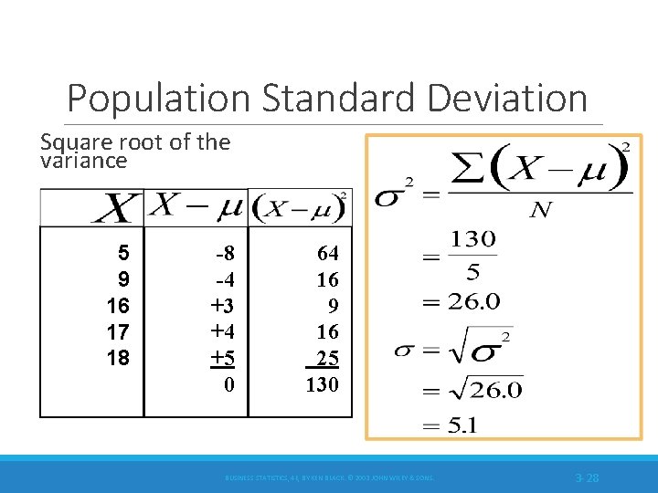
Population Standard Deviation Square root of the variance 5 9 16 17 18 -8 -4 +3 +4 +5 0 64 16 9 16 25 130 BUSINESS STATISTICS, 4 E, BY KEN BLACK. © 2003 JOHN WILEY & SONS. 3 -28
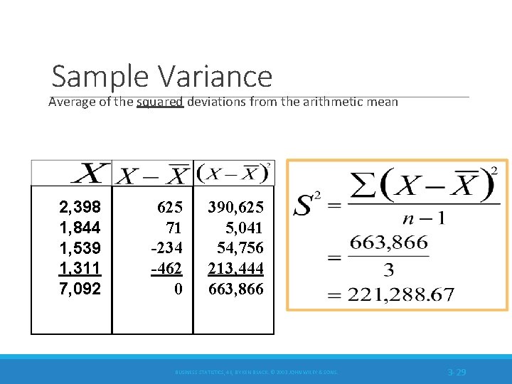
Sample Variance Average of the squared deviations from the arithmetic mean 2, 398 1, 844 1, 539 1, 311 7, 092 625 71 -234 -462 0 390, 625 5, 041 54, 756 213, 444 663, 866 BUSINESS STATISTICS, 4 E, BY KEN BLACK. © 2003 JOHN WILEY & SONS. 3 -29
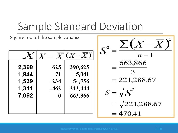
Sample Standard Deviation Square root of the sample variance 2, 398 1, 844 1, 539 1, 311 7, 092 625 71 -234 -462 0 390, 625 5, 041 54, 756 213, 444 663, 866 BUSINESS STATISTICS, 4 E, BY KEN BLACK. © 2003 JOHN WILEY & SONS. 3 -30
Uses of Standard Deviation Indicator of financial risk Quality Control ◦ construction of quality control charts ◦ process capability studies Comparing populations ◦ household incomes in two cities ◦ employee absenteeism at two plants BUSINESS STATISTICS, 4 E, BY KEN BLACK. © 2003 JOHN WILEY & SONS. 3 -31
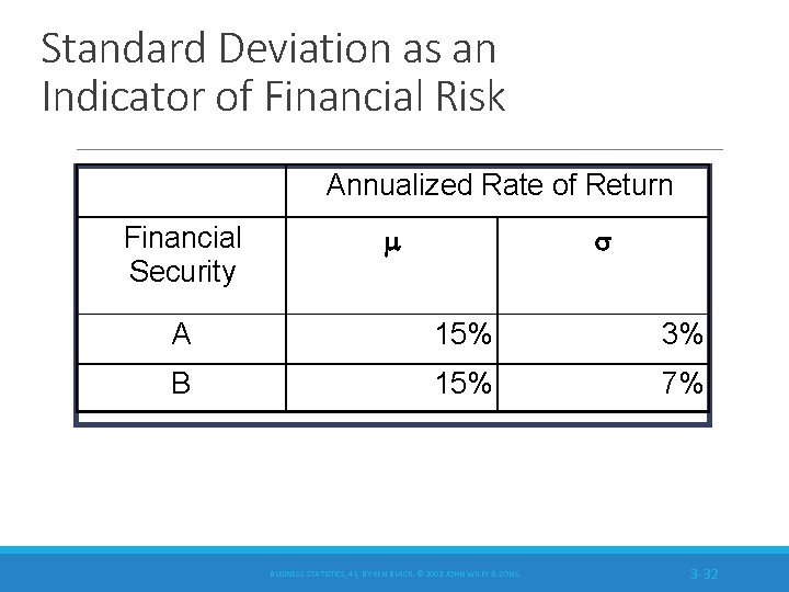
Standard Deviation as an Indicator of Financial Risk Annualized Rate of Return Financial Security A 15% 3% B 15% 7% BUSINESS STATISTICS, 4 E, BY KEN BLACK. © 2003 JOHN WILEY & SONS. 3 -32
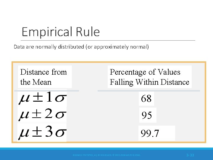
Empirical Rule Data are normally distributed (or approximately normal) Distance from the Mean Percentage of Values Falling Within Distance 68 95 99. 7 BUSINESS STATISTICS, 4 E, BY KEN BLACK. © 2003 JOHN WILEY & SONS. 3 -33

Chebyshev’s Theorem Applies to all distributions BUSINESS STATISTICS, 4 E, BY KEN BLACK. © 2003 JOHN WILEY & SONS. 3 -34

Chebyshev’s Theorem Applies to all distributions Number of Standard Deviations Distance from the Mean Minimum Proportion of Values Falling Within Distance K=2 1 -1/22 = 0. 75 K=3 1 -1/32 = 0. 89 K=4 1 -1/42 = 0. 94 BUSINESS STATISTICS, 4 E, BY KEN BLACK. © 2003 JOHN WILEY & SONS. 3 -35
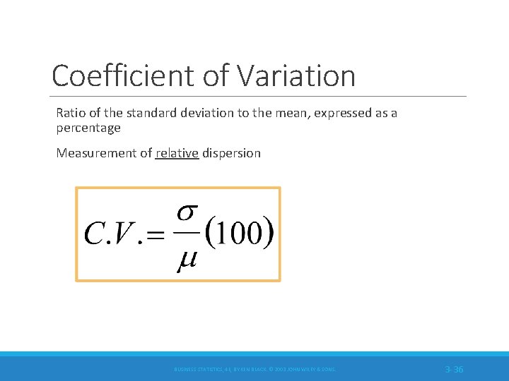
Coefficient of Variation Ratio of the standard deviation to the mean, expressed as a percentage Measurement of relative dispersion BUSINESS STATISTICS, 4 E, BY KEN BLACK. © 2003 JOHN WILEY & SONS. 3 -36
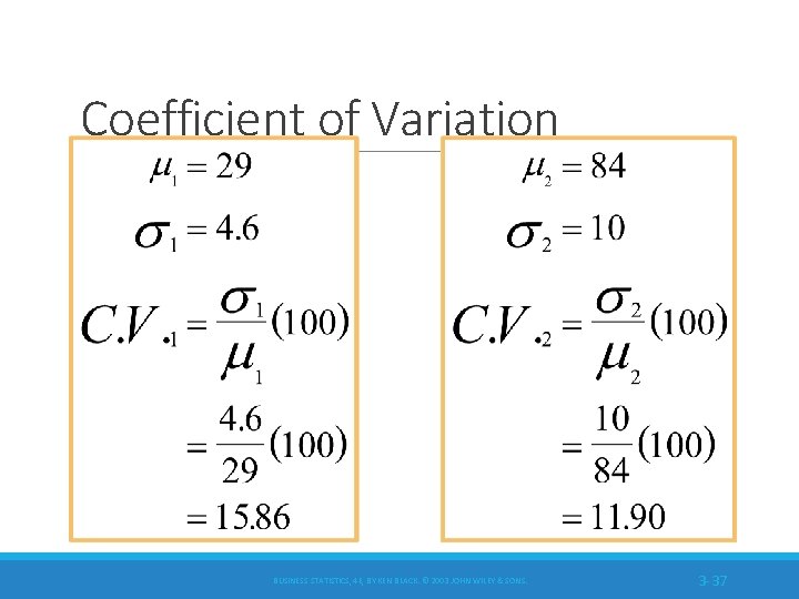
Coefficient of Variation BUSINESS STATISTICS, 4 E, BY KEN BLACK. © 2003 JOHN WILEY & SONS. 3 -37
Measures of Central Tendency and Variability: Grouped Data Measures of Central Tendency ◦ Mean ◦ Median ◦ Mode Measures of Variability ◦ Variance ◦ Standard Deviation BUSINESS STATISTICS, 4 E, BY KEN BLACK. © 2003 JOHN WILEY & SONS. 3 -38
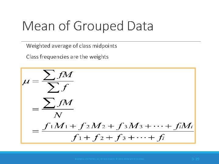
Mean of Grouped Data Weighted average of class midpoints Class frequencies are the weights BUSINESS STATISTICS, 4 E, BY KEN BLACK. © 2003 JOHN WILEY & SONS. 3 -39
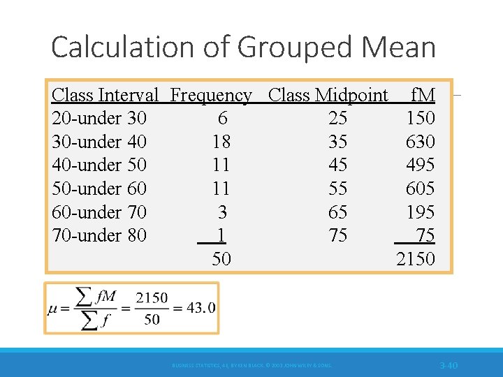
Calculation of Grouped Mean Class Interval Frequency Class Midpoint 20 -under 30 6 25 30 -under 40 18 35 40 -under 50 11 45 50 -under 60 11 55 60 -under 70 3 65 70 -under 80 1 75 50 BUSINESS STATISTICS, 4 E, BY KEN BLACK. © 2003 JOHN WILEY & SONS. f. M 150 630 495 605 195 75 2150 3 -40

Median of Grouped Data BUSINESS STATISTICS, 4 E, BY KEN BLACK. © 2003 JOHN WILEY & SONS. 3 -41
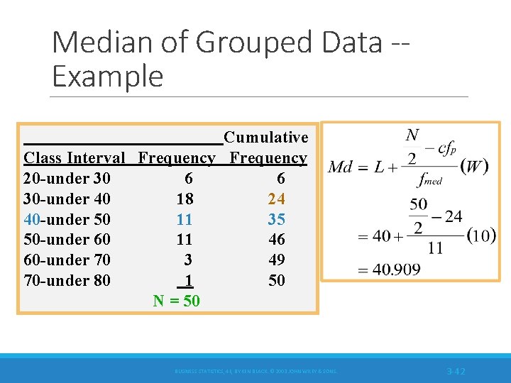
Median of Grouped Data -Example Cumulative Class Interval Frequency 20 -under 30 6 6 30 -under 40 18 24 40 -under 50 11 35 50 -under 60 11 46 60 -under 70 3 49 70 -under 80 1 50 N = 50 BUSINESS STATISTICS, 4 E, BY KEN BLACK. © 2003 JOHN WILEY & SONS. 3 -42
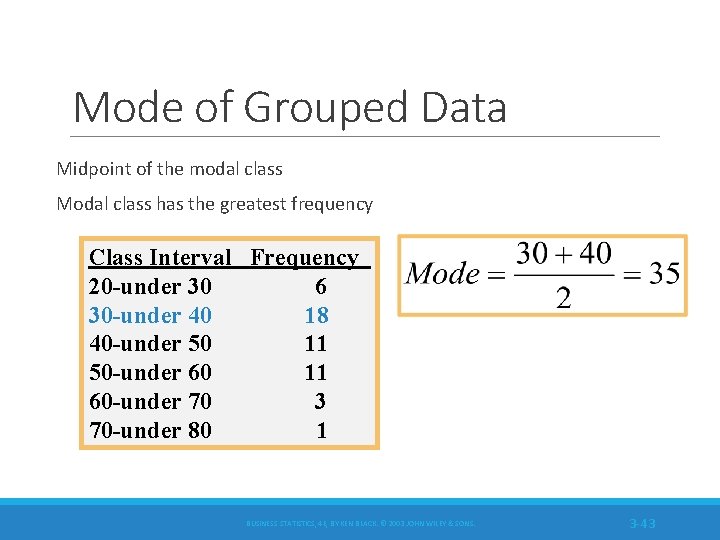
Mode of Grouped Data Midpoint of the modal class Modal class has the greatest frequency Class Interval Frequency 20 -under 30 6 30 -under 40 18 40 -under 50 11 50 -under 60 11 60 -under 70 3 70 -under 80 1 BUSINESS STATISTICS, 4 E, BY KEN BLACK. © 2003 JOHN WILEY & SONS. 3 -43

Variance and Standard Deviation of Grouped Data Population Sample BUSINESS STATISTICS, 4 E, BY KEN BLACK. © 2003 JOHN WILEY & SONS. 3 -44
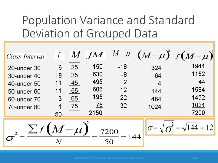
Population Variance and Standard Deviation of Grouped Data 6 18 11 11 3 1 50 150 630 495 605 195 75 2150 -18 -8 2 12 22 32 BUSINESS STATISTICS, 4 E, BY KEN BLACK. © 2003 JOHN WILEY & SONS. 1944 1152 44 1584 1452 1024 7200 3 -45
Measures of Shape Skewness ◦ Absence of symmetry ◦ Extreme values in one side of a distribution Kurtosis ◦ Peakedness of a distribution ◦ Leptokurtic: high and thin ◦ Mesokurtic: normal shape ◦ Platykurtic: flat and spread out Box and Whisker Plots ◦ Graphic display of a distribution ◦ Reveals skewness BUSINESS STATISTICS, 4 E, BY KEN BLACK. © 2003 JOHN WILEY & SONS. 3 -46
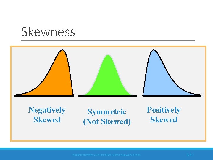
Skewness Negatively Skewed Symmetric (Not Skewed) BUSINESS STATISTICS, 4 E, BY KEN BLACK. © 2003 JOHN WILEY & SONS. Positively Skewed 3 -47
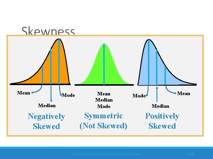
Skewness Mean Median Mode Negatively Skewed Symmetric (Not Skewed) Mode Mean Mode BUSINESS STATISTICS, 4 E, BY KEN BLACK. © 2003 JOHN WILEY & SONS. Median Positively Skewed 3 -48
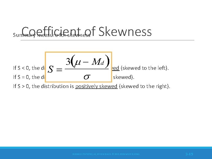
Coefficient of Skewness Summary measure for skewness If S < 0, the distribution is negatively skewed (skewed to the left). If S = 0, the distribution is symmetric (not skewed). If S > 0, the distribution is positively skewed (skewed to the right). BUSINESS STATISTICS, 4 E, BY KEN BLACK. © 2003 JOHN WILEY & SONS. 3 -49
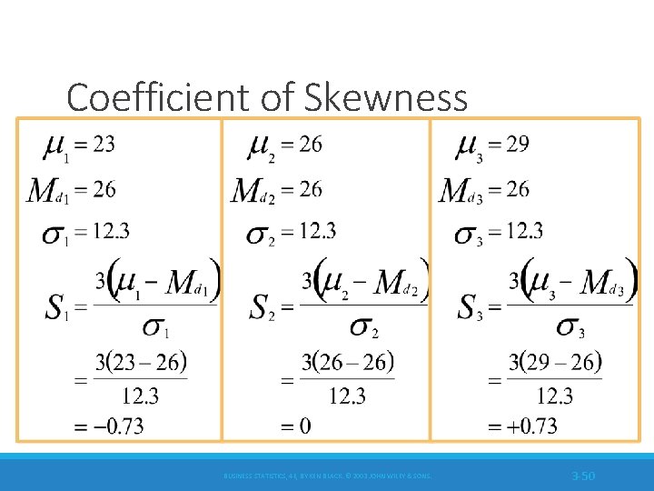
Coefficient of Skewness BUSINESS STATISTICS, 4 E, BY KEN BLACK. © 2003 JOHN WILEY & SONS. 3 -50
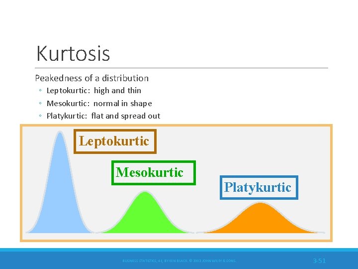
Kurtosis Peakedness of a distribution ◦ Leptokurtic: high and thin ◦ Mesokurtic: normal in shape ◦ Platykurtic: flat and spread out Leptokurtic Mesokurtic Platykurtic BUSINESS STATISTICS, 4 E, BY KEN BLACK. © 2003 JOHN WILEY & SONS. 3 -51
Box and Whisker Plot Five secific values are used: ◦ Median, Q 2 ◦ First quartile, Q 1 ◦ Third quartile, Q 3 ◦ Minimum value in the data set ◦ Maximum value in the data set Inner Fences ◦ IQR = Q 3 - Q 1 ◦ Lower inner fence = Q 1 - 1. 5 IQR ◦ Upper inner fence = Q 3 + 1. 5 IQR Outer Fences ◦ Lower outer fence = Q 1 - 3. 0 IQR ◦ Upper outer fence = Q 3 + 3. 0 IQR BUSINESS STATISTICS, 4 E, BY KEN BLACK. © 2003 JOHN WILEY & SONS. 3 -52
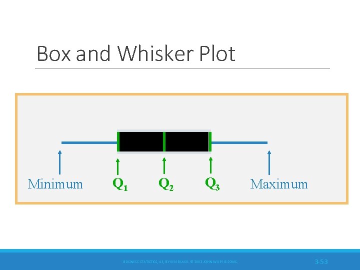
Box and Whisker Plot Minimum Q 1 Q 2 Q 3 BUSINESS STATISTICS, 4 E, BY KEN BLACK. © 2003 JOHN WILEY & SONS. Maximum 3 -53
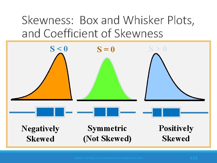
Skewness: Box and Whisker Plots, and Coefficient of Skewness S<0 Negatively Skewed S=0 Symmetric (Not Skewed) BUSINESS STATISTICS, 4 E, BY KEN BLACK. © 2003 JOHN WILEY & SONS. S>0 Positively Skewed 3 -54

Pearson Product-Moment Correlation Coefficient BUSINESS STATISTICS, 4 E, BY KEN BLACK. © 2003 JOHN WILEY & SONS. 3 -55
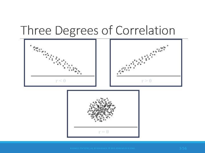
Three Degrees of Correlation BUSINESS STATISTICS, 4 E, BY KEN BLACK. © 2003 JOHN WILEY & SONS. 3 -56
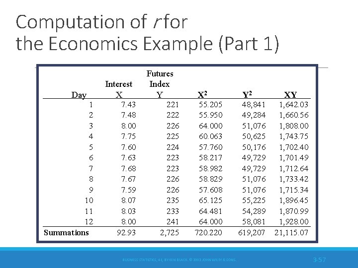
Computation of r for the Economics Example (Part 1) Day 1 2 3 4 5 6 7 8 9 10 11 12 Summations Interest X 7. 43 7. 48 8. 00 7. 75 7. 60 7. 63 7. 68 7. 67 7. 59 8. 07 8. 03 8. 00 92. 93 Futures Index Y 221 222 226 225 224 223 226 235 233 241 2, 725 X 2 55. 205 55. 950 64. 000 60. 063 57. 760 58. 217 58. 982 58. 829 57. 608 65. 125 64. 481 64. 000 720. 220 BUSINESS STATISTICS, 4 E, BY KEN BLACK. © 2003 JOHN WILEY & SONS. Y 2 48, 841 49, 284 51, 076 50, 625 50, 176 49, 729 51, 076 55, 225 54, 289 58, 081 619, 207 XY 1, 642. 03 1, 660. 56 1, 808. 00 1, 743. 75 1, 702. 40 1, 701. 49 1, 712. 64 1, 733. 42 1, 715. 34 1, 896. 45 1, 870. 99 1, 928. 00 21, 115. 07 3 -57

Computation of r for the Economics Example (Part 2) BUSINESS STATISTICS, 4 E, BY KEN BLACK. © 2003 JOHN WILEY & SONS. 3 -58
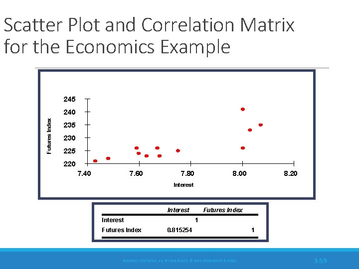
Scatter Plot and Correlation Matrix for the Economics Example 245 Futures Index 240 235 230 225 220 7. 40 7. 60 7. 80 8. 00 8. 20 Interest Futures Index 1 0. 815254 BUSINESS STATISTICS, 4 E, BY KEN BLACK. © 2003 JOHN WILEY & SONS. 1 3 -59
- Slides: 59