Chapter 3 Describing Data Using Numerical Measures Fall

Chapter 3 Describing Data Using Numerical Measures Fall 2006 – Fundamentals of Business Statistics 1

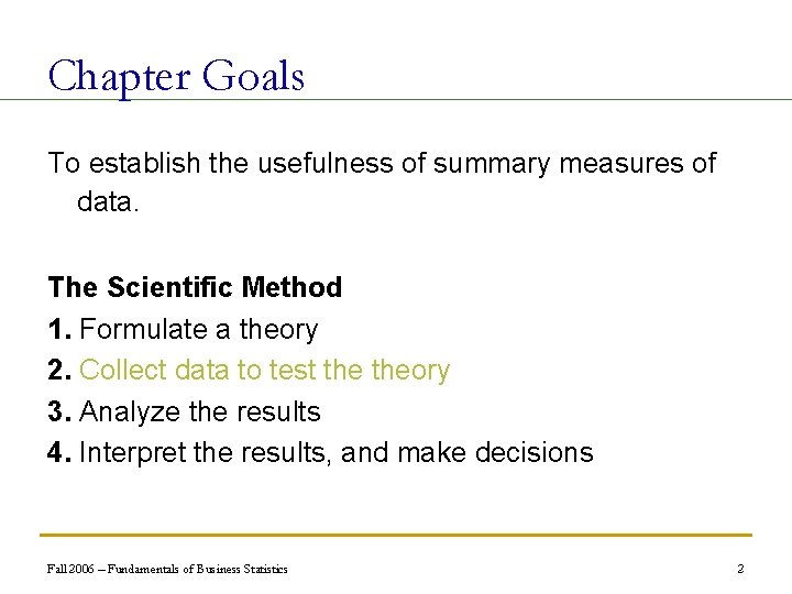
Chapter Goals To establish the usefulness of summary measures of data. The Scientific Method 1. Formulate a theory 2. Collect data to test theory 3. Analyze the results 4. Interpret the results, and make decisions Fall 2006 – Fundamentals of Business Statistics 2

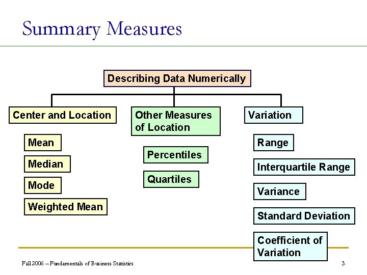
Summary Measures Describing Data Numerically Center and Location Other Measures of Location Mean Median Mode Weighted Mean Variation Range Percentiles Interquartile Range Quartiles Variance Standard Deviation Coefficient of Variation Fall 2006 – Fundamentals of Business Statistics 3

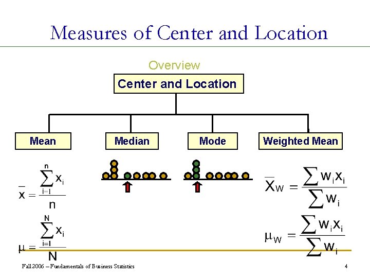
Measures of Center and Location Overview Center and Location Mean Median Fall 2006 – Fundamentals of Business Statistics Mode Weighted Mean 4

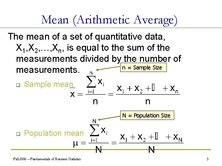
Mean (Arithmetic Average) The mean of a set of quantitative data, X 1, X 2, …, Xn, is equal to the sum of the measurements divided by the number of n = Sample Size measurements. q Sample mean N = Population Size q Population mean Fall 2006 – Fundamentals of Business Statistics 5

Example Find the mean of the following 5 numbers 5, 3, 8, 5, 6 Fall 2006 – Fundamentals of Business Statistics 6

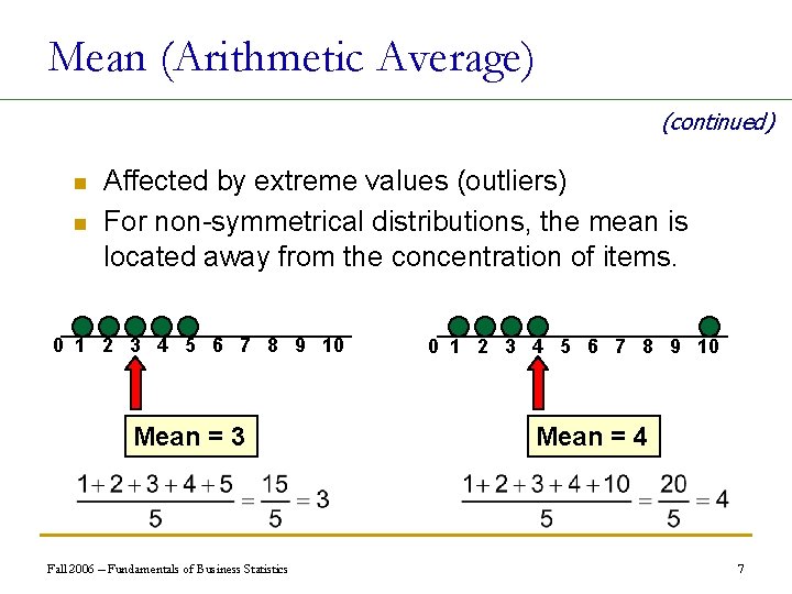
Mean (Arithmetic Average) (continued) n n Affected by extreme values (outliers) For non-symmetrical distributions, the mean is located away from the concentration of items. 0 1 2 3 4 5 6 7 8 9 10 Mean = 3 Fall 2006 – Fundamentals of Business Statistics 0 1 2 3 4 5 6 7 8 9 10 Mean = 4 7

YDI 5. 1 and 5. 2 n Kim’s test scores are 7, 98, 25, 19, and 26. Calculate Kim’s mean test score. Does the mean do a good job of capturing Kim’s test scores? n The mean score for 3 students is 54, and the mean score for 4 different students is 76. What is the mean score for all 7 students? Fall 2006 – Fundamentals of Business Statistics 8

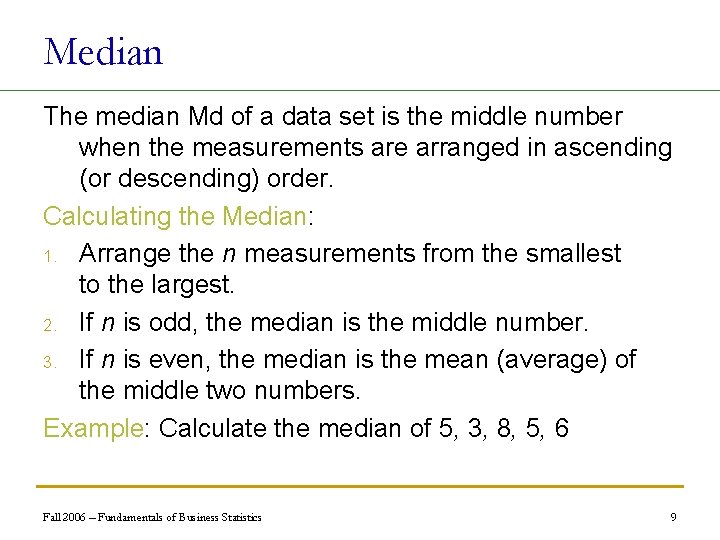
Median The median Md of a data set is the middle number when the measurements are arranged in ascending (or descending) order. Calculating the Median: 1. Arrange the n measurements from the smallest to the largest. 2. If n is odd, the median is the middle number. 3. If n is even, the median is the mean (average) of the middle two numbers. Example: Calculate the median of 5, 3, 8, 5, 6 Fall 2006 – Fundamentals of Business Statistics 9

Median n Not affected by extreme values 0 1 2 3 4 5 6 7 8 9 10 Median = 3 n In an ordered array, the median is the “middle” number. What if the values in the data set are repeated? Fall 2006 – Fundamentals of Business Statistics 10

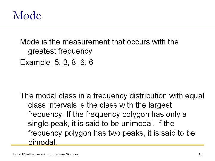
Mode is the measurement that occurs with the greatest frequency Example: 5, 3, 8, 6, 6 The modal class in a frequency distribution with equal class intervals is the class with the largest frequency. If the frequency polygon has only a single peak, it is said to be unimodal. If the frequency polygon has two peaks, it is said to be bimodal. Fall 2006 – Fundamentals of Business Statistics 11

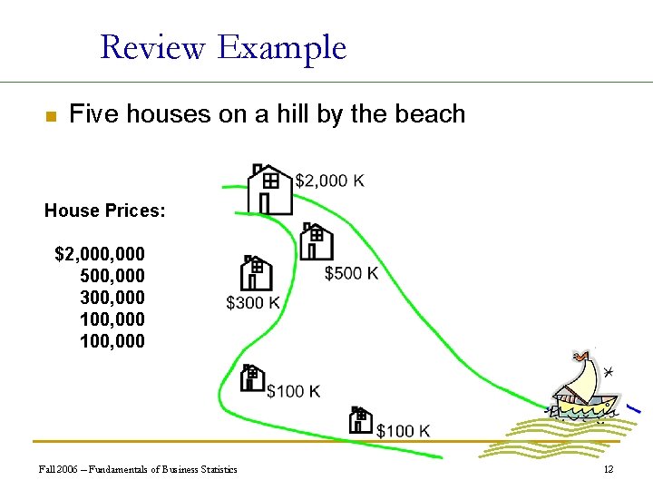
Review Example n Five houses on a hill by the beach House Prices: $2, 000 500, 000 300, 000 100, 000 Fall 2006 – Fundamentals of Business Statistics 12

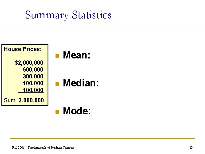
Summary Statistics House Prices: $2, 000 500, 000 300, 000 100, 000 n Mean: n Median: n Mode: Sum 3, 000 Fall 2006 – Fundamentals of Business Statistics 13

Which measure of location is the “best”? n Mean is generally used, unless extreme values (outliers) exist n Then median is often used, since the median is not sensitive to extreme values. q Example: Median home prices may be reported for a region – less sensitive to outliers Fall 2006 – Fundamentals of Business Statistics 14

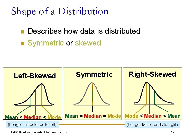
Shape of a Distribution n Describes how data is distributed n Symmetric or skewed Left-Skewed Symmetric Right-Skewed Mean < Median < Mode Mean = Median = Mode < Median < Mean (Longer tail extends to left) Fall 2006 – Fundamentals of Business Statistics (Longer tail extends to right) 15

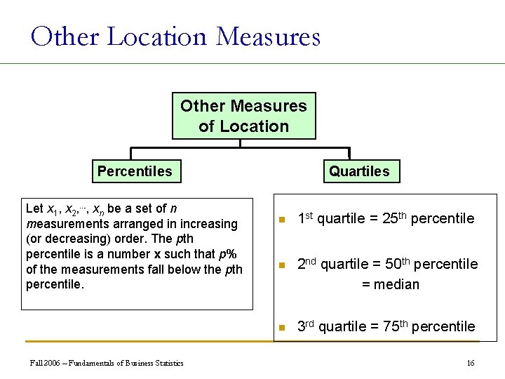
Other Location Measures Other Measures of Location Percentiles Let x 1, x 2, ⋯, xn be a set of n measurements arranged in increasing (or decreasing) order. The pth percentile is a number x such that p% of the measurements fall below the pth percentile. Fall 2006 – Fundamentals of Business Statistics Quartiles n 1 st quartile = 25 th percentile n 2 nd quartile = 50 th percentile = median n 3 rd quartile = 75 th percentile 16

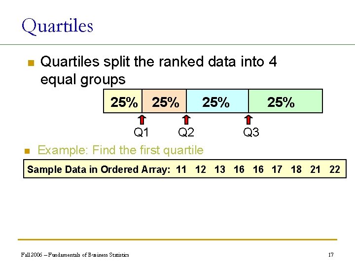
Quartiles n Quartiles split the ranked data into 4 equal groups 25% n 25% Q 1 Q 2 Example: Find the first quartile 25% Q 3 Sample Data in Ordered Array: 11 12 13 16 16 17 18 21 22 Fall 2006 – Fundamentals of Business Statistics 17

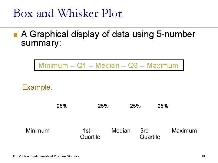
Box and Whisker Plot n A Graphical display of data using 5 -number summary: Minimum -- Q 1 -- Median -- Q 3 -- Maximum Example: 25% Fall 2006 – Fundamentals of Business Statistics 25% 25% 18

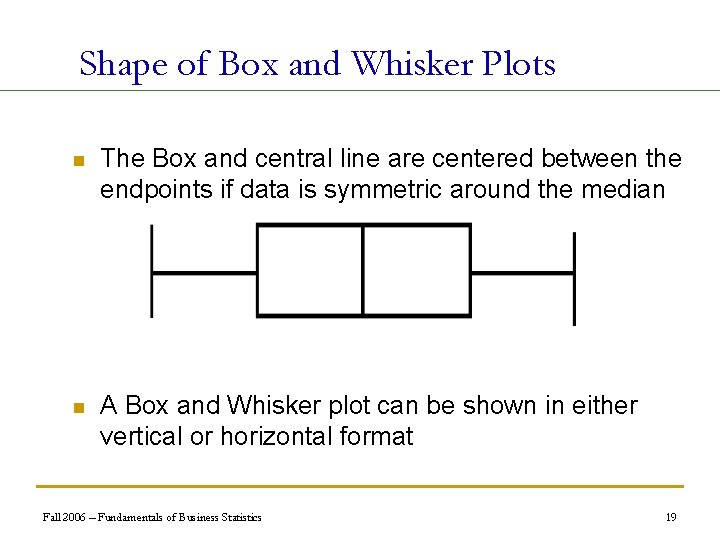
Shape of Box and Whisker Plots n The Box and central line are centered between the endpoints if data is symmetric around the median n A Box and Whisker plot can be shown in either vertical or horizontal format Fall 2006 – Fundamentals of Business Statistics 19

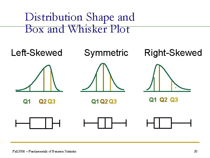
Distribution Shape and Box and Whisker Plot Left-Skewed Q 1 Q 2 Q 3 Fall 2006 – Fundamentals of Business Statistics Symmetric Q 1 Q 2 Q 3 Right-Skewed Q 1 Q 2 Q 3 20

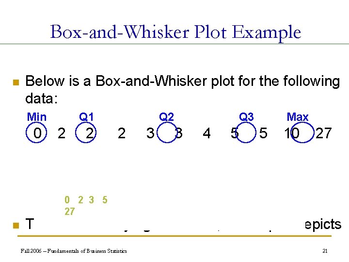
Box-and-Whisker Plot Example n Below is a Box-and-Whisker plot for the following data: Min 0 Q 1 2 2 Q 2 2 3 Q 3 3 4 5 Max 5 10 27 0 2 3 5 27 n This data is very right skewed, as the plot depicts Fall 2006 – Fundamentals of Business Statistics 21

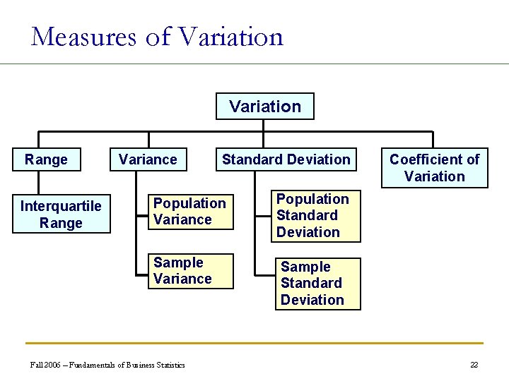
Measures of Variation Range Interquartile Range Variance Standard Deviation Population Variance Population Standard Deviation Sample Variance Sample Standard Deviation Fall 2006 – Fundamentals of Business Statistics Coefficient of Variation 22

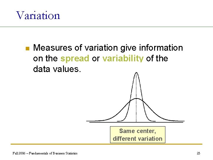
Variation n Measures of variation give information on the spread or variability of the data values. Same center, different variation Fall 2006 – Fundamentals of Business Statistics 23

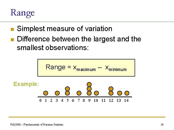
Range n n Simplest measure of variation Difference between the largest and the smallest observations: Range = xmaximum – xminimum Example: 0 1 2 3 4 5 6 7 8 9 10 11 12 13 14 Fall 2006 – Fundamentals of Business Statistics 24

Disadvantages of the Range n n Considers only extreme values With a frequency distribution, the range of original data cannot be determined exactly. Fall 2006 – Fundamentals of Business Statistics 25

Interquartile Range n Can eliminate some outlier problems by using the interquartile range n Eliminate some high-and low-valued observations and calculate the range from the remaining values. n Interquartile range = 3 rd quartile – 1 st quartile Fall 2006 – Fundamentals of Business Statistics 26

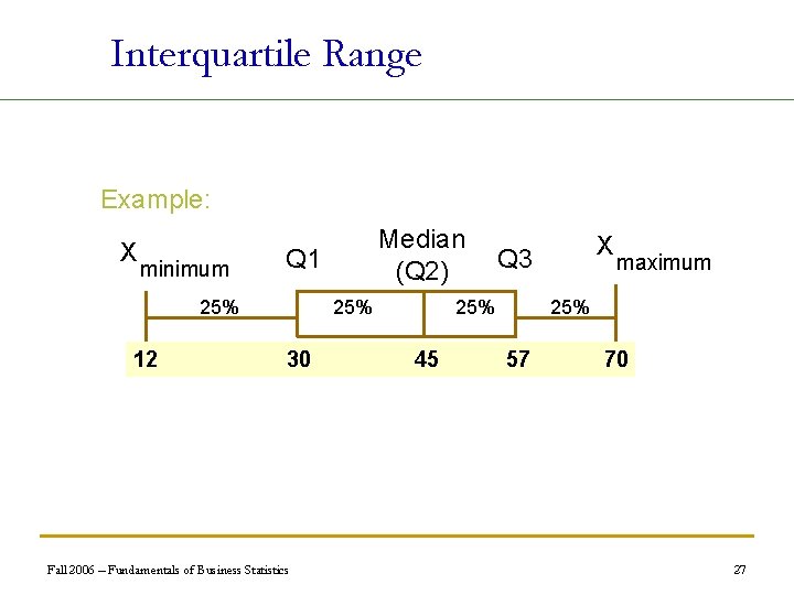
Interquartile Range Example: X minimum Q 1 25% 12 Median (Q 2) 25% 30 Fall 2006 – Fundamentals of Business Statistics 25% 45 X Q 3 maximum 25% 57 70 27

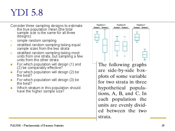
YDI 5. 8 Consider three sampling designs to estimate the true population mean (the total sample size is the same for all three designs): 1. simple random sampling 2. stratified random sampling taking equal sample sizes from the two strata 3. stratified random sampling taking most units from one strata, but sampling a few units from the other strata n For which population will design (1) and (2) be comparably effective? n For which population will design (2) be the best? n For which population will design (3) be the best? n Which stratum in this population should have the higher sample size? Fall 2006 – Fundamentals of Business Statistics 28

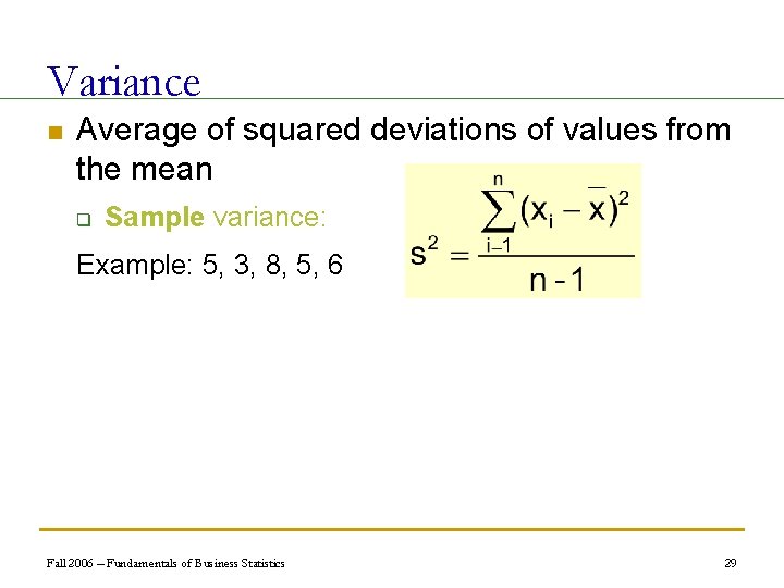
Variance n Average of squared deviations of values from the mean q Sample variance: Example: 5, 3, 8, 5, 6 Fall 2006 – Fundamentals of Business Statistics 29

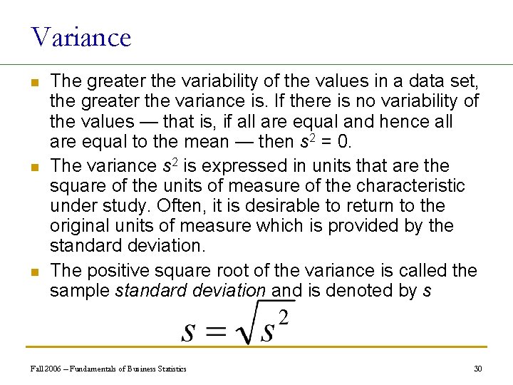
Variance n n n The greater the variability of the values in a data set, the greater the variance is. If there is no variability of the values — that is, if all are equal and hence all are equal to the mean — then s 2 = 0. The variance s 2 is expressed in units that are the square of the units of measure of the characteristic under study. Often, it is desirable to return to the original units of measure which is provided by the standard deviation. The positive square root of the variance is called the sample standard deviation and is denoted by s Fall 2006 – Fundamentals of Business Statistics 30

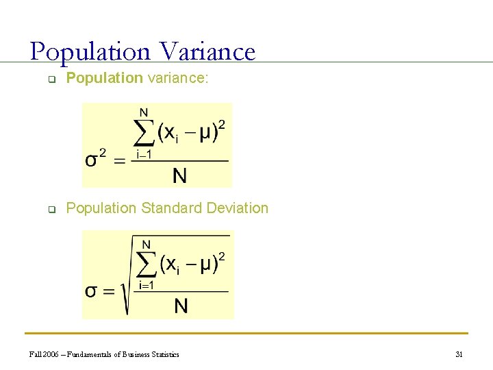
Population Variance q Population variance: q Population Standard Deviation Fall 2006 – Fundamentals of Business Statistics 31

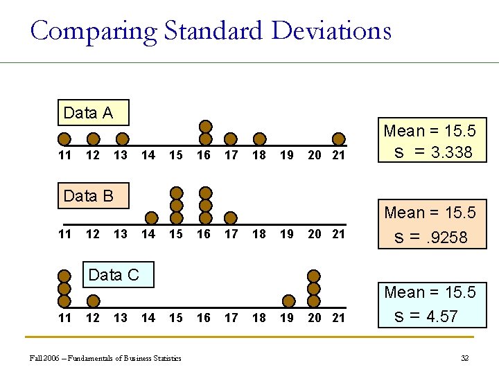
Comparing Standard Deviations Data A 11 12 13 14 15 16 17 18 19 20 21 Mean = 15. 5 s = 3. 338 20 21 Mean = 15. 5 s =. 9258 20 21 Mean = 15. 5 s = 4. 57 Data B 11 12 13 14 15 16 17 18 19 Data C 11 12 13 14 15 Fall 2006 – Fundamentals of Business Statistics 16 17 18 19 32

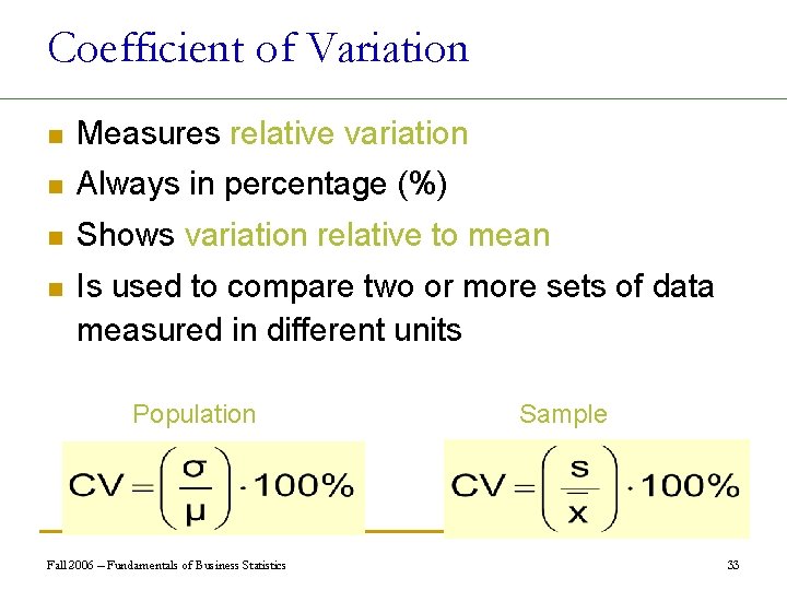
Coefficient of Variation n Measures relative variation n Always in percentage (%) n Shows variation relative to mean n Is used to compare two or more sets of data measured in different units Population Fall 2006 – Fundamentals of Business Statistics Sample 33

YDI n Stock A: q Average price last year = $50 q Standard deviation = $5 n Stock B: q q Average price last year = $100 Standard deviation = $5 Fall 2006 – Fundamentals of Business Statistics 34

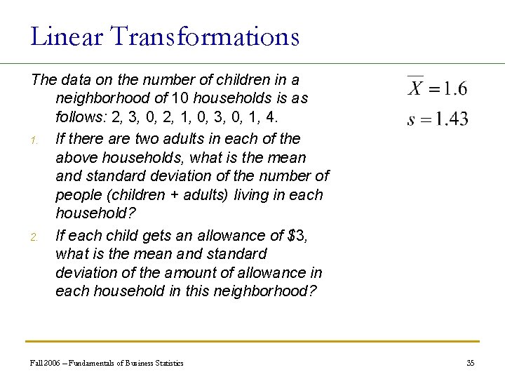
Linear Transformations The data on the number of children in a neighborhood of 10 households is as follows: 2, 3, 0, 2, 1, 0, 3, 0, 1, 4. 1. If there are two adults in each of the above households, what is the mean and standard deviation of the number of people (children + adults) living in each household? 2. If each child gets an allowance of $3, what is the mean and standard deviation of the amount of allowance in each household in this neighborhood? Fall 2006 – Fundamentals of Business Statistics 35

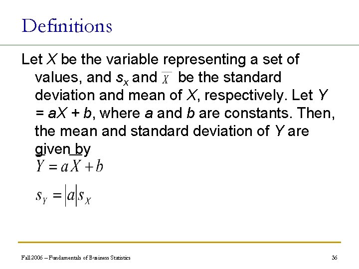
Definitions Let X be the variable representing a set of values, and sx and be the standard deviation and mean of X, respectively. Let Y = a. X + b, where a and b are constants. Then, the mean and standard deviation of Y are given by Fall 2006 – Fundamentals of Business Statistics 36

Standardized Data Values n A standardized data value refers to the number of standard deviations a value is from the mean n Standardized data values are sometimes referred to as z-scores Fall 2006 – Fundamentals of Business Statistics 37

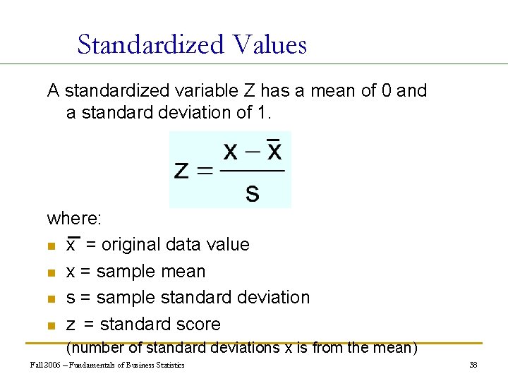
Standardized Values A standardized variable Z has a mean of 0 and a standard deviation of 1. where: n x = original data value n x = sample mean n s = sample standard deviation n z = standard score (number of standard deviations x is from the mean) Fall 2006 – Fundamentals of Business Statistics 38

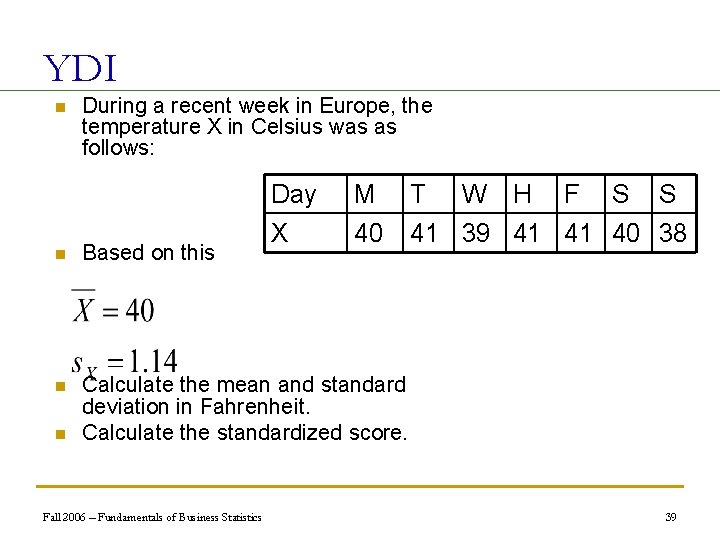
YDI n During a recent week in Europe, the temperature X in Celsius was as follows: Day X M 40 n Based on this n Calculate the mean and standard deviation in Fahrenheit. Calculate the standardized score. n Fall 2006 – Fundamentals of Business Statistics T W H F S S 41 39 41 41 40 38 39