Chapter 3 Decisions Involving Multiple Objectives SMART 1

Chapter 3 Decisions Involving Multiple Objectives: SMART 1

Objectives and Attributes An objective = an indication of preferred direction of movement, i. e. ‘minimize’ or ‘maximize’ Minimize costs or maximize market share n 2

n n An attribute is used to measure performance in relation to an objective the objective 'maximize the exposure of a television advertisement' the attribute 'number of people surveyed who recall seeing the advertisement' proxy attribute 3

Value and utility n n If the decision involves no element of risk and uncertainty we will refer to this score as the value of the course of action. Alternatively, where the decision involves risk and uncertainty, we will refer to this score as the utility of the course of action. 4

n n The following problem will be used to illustrate the analysis of decisions involving multiple objectives. The owner of the business is considering seven possible new offices, all of which would be rented. 5

An office location problem Location of office Annual rent ($) Addison Square (A) 30 000 Bilton Village (B) 15 000 Carlisle Walk (C) 5 000 Denver Street (D) 12 000 Elton Street (E) 30 000 Filton Village (F) 15 000 Gorton Square (G) 10 000 6

An overview of the analysis n n Simple Multi attribute Rating Technique (SMART) The analysis involved is transparent, so the method is likely to yield an enhanced understanding of the problem and be acceptable to the decision maker who is distrustful of a mathematical 'black box' approach. 7

Main stages of SMART 1 Identify decision maker(s) 2 Identify alternative courses of action 3 Identify the relevant attributes 4 Assess the performance of the alternatives on each attribute 5 Determine a weight for each attribute 6 For each alternative, take a weighted average of the values assigned to that alternative 7 Make a provisional decision 8 Perform sensitivity analysis 8

n n Stage 1: Identify the decision maker (or decision makers). In this problem we will assume that this is just the business owner, but probably the application of SMART could be on the problems involving groups of decision makers. 9

n n Stage 2: Identify the alternative courses of action. In this problem these are, of course, represented by the different offices the owner can choose. 10

n n Stage 3: ldentify the attributes which are relevant to the decision problem. The attributes which distinguish the different offices will be factors such as rent, size and quality of working conditions. A value tree can be of use when identifying relevant attributes. 11

Stage 4: For each attribute, assign values to measure the performance of the alternatives on that attribute. For example, how well do the offices compare when considering the quality of the working conditions they offer? n 12

n n Stage 5: Determine a weight for each attribute. This may reflect how important the attribute is to the decision maker. 13

n Stage 6: For each alternative, take a weighted average of the values assigned to that alternative. n This will give us a measure of how well an office performs over all the attributes. 14

n Stage 7: Make a provisional decision. 15

n Stage 8: Perform sensitivity analysis to see how robust the decision is to changes in the figures supplied by the decision maker. 16

n n We need a set of attributes which can be assessed on a numeric scale. A value tree can be useful. 17

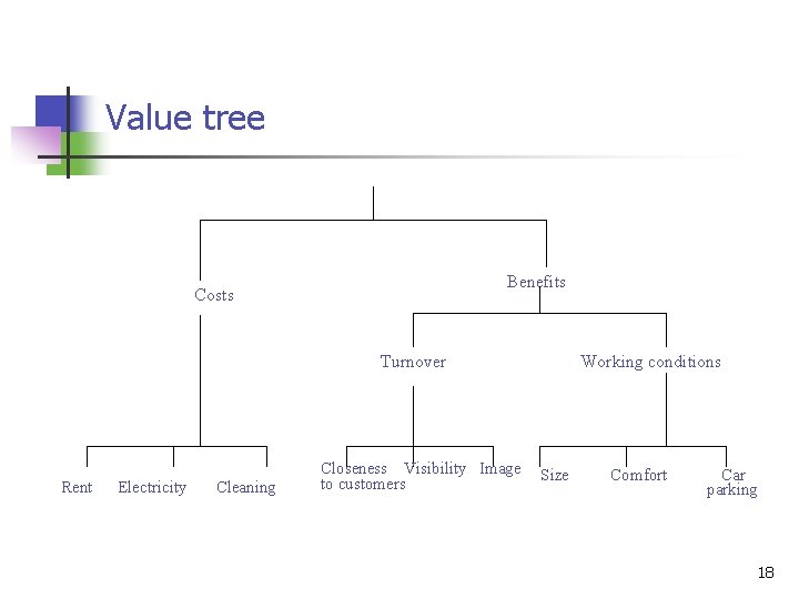
Value tree Benefits Costs Turnover Rent Electricity Cleaning Closeness Visibility Image to customers Working conditions Size Comfort Car parking 18

n n costs and benefits Having established the main attributes for our business owner, we need to decompose them to a level where they can be assessed. 19

n n Three main costs that are of concern to him: the annual rent, the cost of electricity and the cost of having the office regularly cleaned. Benefits can be subdivided into ‘potential for improved turnover’ and ‘staff working conditions’ 20

Potential for improved turnover n Attributes to be ‘the closeness of the office to potential customers’, ‘the visibility of the site’ (much business is generated from people who see the office while passing by) and ‘the image of the location’ (a decaying building in a back street may convey a poor image and lead to a loss of business). 21

Staff working conditions n ‘size’, ‘comfort’ and ‘car parking facilities’ 22

Is the value tree an accurate and useful representation of the decision maker’s concerns? 1. Completeness 2. Operationality 3. Decomposability 4. Absence of redundancy 5. Minimum size 23

Completeness n If the tree is complete, all the attributes which are of concern to the decision maker will have been included. 24

Operationality n This criterion is met when all the lowest level attri butes in the tree are specific enough for the decision maker to evaluate and compare them for the different options. 25

Decomposability n This criterion requires that the performance of an option on one attribute can be judged independently of its performance on other attributes 26

Absence of redundancy n n If two attributes duplicate each other because they actually represent the same thing then one of these attributes is clearly redundant. One way of identifying redundancy is to establish whether the decision would in any way be affected if a given attribute was eliminated from the tree. 27

Minimum size n n If the tree is too large any meaningful analysis may be impossible. To ensure that this does not happen, attributes should not be decomposed beyond the level where they can be evaluated. 28

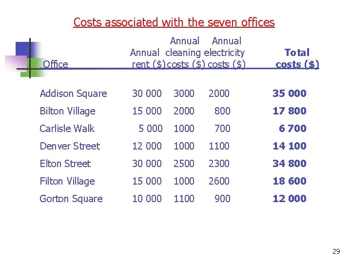
Costs associated with the seven offices Office Annual Annual cleaning electricity Total rent ($) costs ($) Addison Square 30 000 3000 2000 35 000 Bilton Village 15 000 2000 800 17 800 Carlisle Walk 5 000 1000 700 6 700 Denver Street 12 000 1100 14 100 Elton Street 30 000 2500 2300 34 800 Filton Village 15 000 1000 2600 18 600 Gorton Square 10 000 1100 900 12 000 29

Measuring how well the options perform on each attribute n n In measuring these attributes our task will be made easier if we can identify variables to represent the attributes. There are two alternative approaches which can be used to measure the performance of the offices on each attribute: direct rating and the use of value functions. 30

Direct rating n Consider those attributes which cannot be represented by easily quantifiable variables, such as “image”. 31

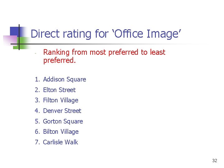
Direct rating for ‘Office Image’ Ranking from most preferred to least preferred. 1. Addison Square 2. Elton Street 3. Filton Village 4. Denver Street 5. Gorton Square 6. Bilton Village 7. Carlisle Walk 32

n n Addison Square, the best location for image, can now be given a value for image of 100 and Carlisle Walk, the location with the least appealing image, can be given a value of 0. The use of 0 and 100 makes the judgments which follow much easier and it also simplifies the arithmetic. 33

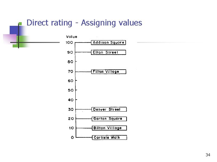
n Direct rating Assigning values 34

n n Note that it is the interval (or improvement) between the points in the scale which we compare. We cannot say that the image of Gorton Square is twice as preferable as that of the Bilton Village office. 35

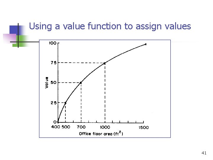
Value functions n n Consider the benefit attributes which can be represented by easily quantified variables. First, we need to measure the owner's relative strength of preference for offices of different sizes. (refer to Page 37) 36

n n To translate the floor areas into values. The owner judges that the larger the office, the more attractive it is. In mathematical notation we can say that: v(1500) = 100 37

n n n We now need to find the value of the office areas which fall between the most preferred and least preferred areas. There are several methods which can be used to elicit a value function, but one of the most widely applied is bisection. This method requires the owner to identify an office area whose value is halfway between the least preferred area (400 ft 2) and the most preferred area (1500 ft 2). 38

n n n Finally, he agrees that 700 ft 2 has the midpoint value, so v(700) = 50. Having identified the midpoint value, the decision maker is now asked to identify the 'quarter points'. v(500) = 25; v(1000) = 75. 39

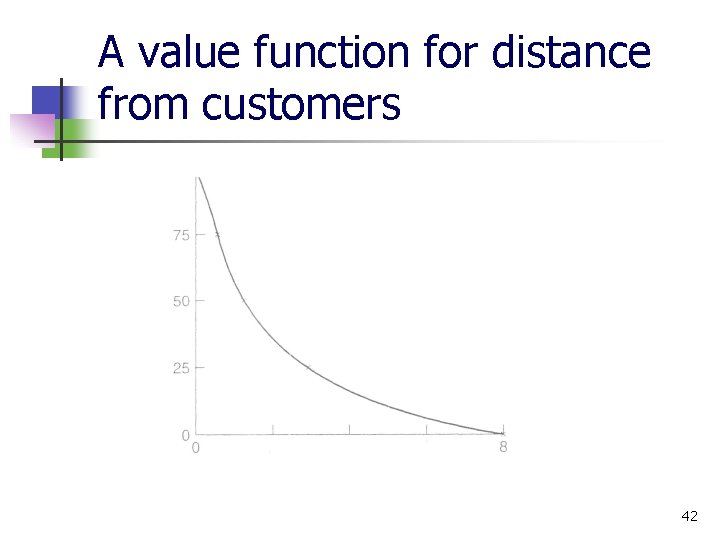
n A similar method can be applied to the attribute 'closeness to cus tomers'. This attribute has been represented by the variable ‘distance from town center’ and the value function is shown in Figure 3. 4. 40

Using a value function to assign values 41

A value function for distance from customers 42

Values for the office location problem 43

Determining the weights of the attributes n n n In order to make a decision the owner now needs to combine the values for the different attributes in order to gain a view of the overall benefits which each office has to offer. An intuitively appealing way of achieving this is to attach weights to each of the attributes that reflect their importance to the decision maker. Unfortunately, this approach can lead to serious problems. 44

n n The problem with importance weights is that they may not take into account the range between the least and most preferred options on each attribute. The range between worst and best is small, then this attribute is unlikely to be important in the decision, even though the decision maker may consider it to be an important attribute per se. 45

n This problem can be avoided by using swing weights. n These are derived by asking the decision maker to compare a change (or swing) from the least preferred to the most preferred value on one attribute to a similar change in another attribute. 46

n n n n The owner's rankings (closeness) are: (1) Closeness to customers (2) Visibility (3) Image (4) Size (5) Comfort (6) Car parking facilities 47

n n We can now give 'closeness to customers 7 a weight of 100. The swing in 'visibility' is 80% as important as the swing in 'closeness to customers', so visibility is given a weight of 80. The importance of the other attributes can then be determined in the same way. 48

For example. . . A swing from the worst ‘image’ to the best ‘image’ is considered to be 70% as important as a swing from the worst to the best location for ‘closeness to customers’ . . . so ‘image’ is assigned a weight of 70. 49

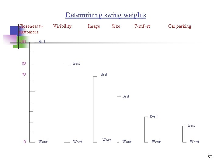
Determining swing weights Closeness to customers 100 Visibility Image Size Comfort Car parking Best 80 Best 70 Best 0 Worst Worst 50

n Normalization is achieved by simply dividing each weight by the sum of the weights (310) and multiplying by 100. (Refer to Page 42) 51

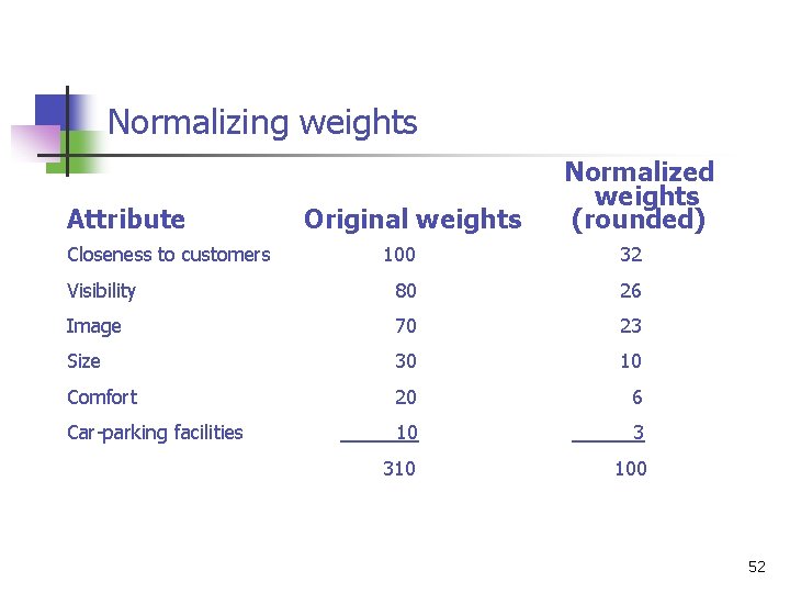
Normalizing weights Attribute Original weights Normalized weights (rounded) Closeness to customers 100 32 Visibility 80 26 Image 70 23 Size 30 10 Comfort 20 6 10 3 310 100 Car parking facilities 52

Aggregating the benefits using the additive model n n Assume that the additive model is appropriate. The additive model is by far the most widely used, but it is not suitable for all circumstances. In particular, the model is inappropriate where there is an interaction between the values associ ated with some of the attributes. 53

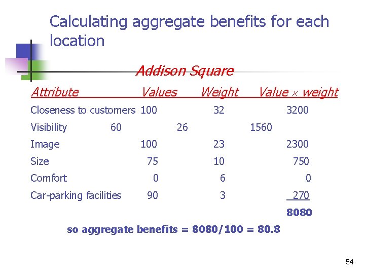
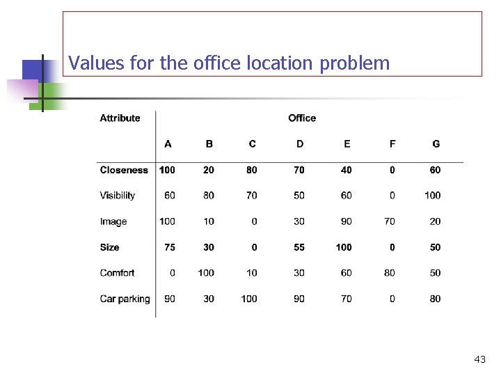
Calculating aggregate benefits for each location Addison Square Attribute Values Closeness to customers 100 Visibility 60 Weight Value weight 32 3200 26 1560 Image 100 23 2300 Size 75 10 750 Comfort 0 6 Car parking facilities 90 3 0 270 8080 so aggregate benefits = 8080/100 = 80. 8 54

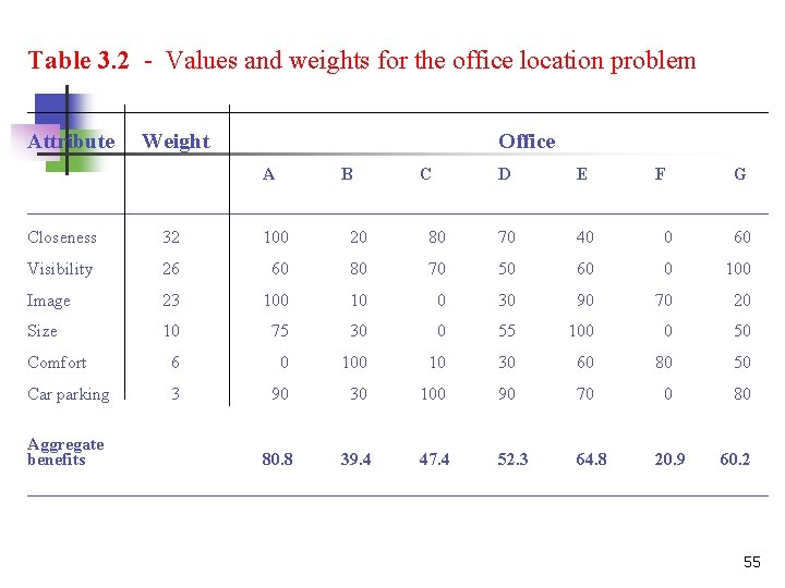
Table 3. 2 - Values and weights for the office location problem __________________________________ Attribute Weight Office A B C D E F G ___________________________________________ Closeness 32 100 20 80 70 40 0 60 Visibility 26 60 80 70 50 60 0 100 Image 23 100 10 0 30 90 70 20 Size 10 75 30 0 55 100 0 50 Comfort 6 0 10 30 60 80 50 Car parking 3 90 30 100 90 70 0 80 80. 8 39. 4 47. 4 52. 3 64. 8 Aggregate benefits 20. 9 60. 2 ___________________________________________ 55

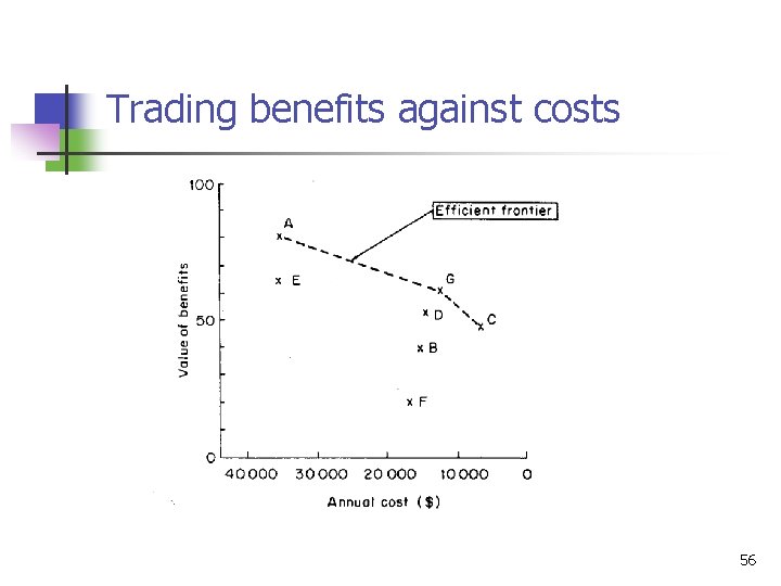
Trading benefits against costs 56

n n The higher an office appears on the benefits scale and the further to the right on the cost scale, the more attractive it will be. the only locations which are worth considering are Addison Square (A), Gorton Square (G) and Carlisle Walk (C). These non dominated offices are said to lie on the efficient frontier. 57

n n The choice between the three offices on the efficient frontier will depend on the relative weight the owner attaches to costs and benefits. The decision maker may think that a more formal approach would help him. 58

n n n The increment value between the efficient frontiers $414 per extra point and 1117 per extra point The image; the owner is prepared to pay $15000 to gain 23 points in the value of aggregate benefits. This implies that he is prepared to pay $15 000/23 or $652 per point. On this basis he should choose the Gorton Square office. 59

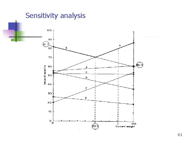
Sensitivity analysis n n Sensitivity analysis is used to examine how robust the choice of an alternative is to changes in the figures used in the analysis. The owner is a little worried about the weight of turnover (i. e. 81) relative to working conditions (i. e. 19) and he would like to know what would happen if this weight was changed. 60

Sensitivity analysis 61

Theoretical considerations n The axioms of the method n n n Decidability Transitivity Summation Solvability Finite upper and lower bounds for value 62

Assumptions made when aggregating values n n The additive model is used to aggregate the values for the different attributes. The use of this model is not appropriate where there is an interaction between the scores on the attributes. In order to apply the model we need to assume that mutual preference independence exists between the attributes. 63

Mutual preference independence does not exist n n Maybe the decision maker considers image only to be of value if the office is highly visible. If image is not preference independent of visibility, the additive model will not correctly represent the owner's preferences. 64

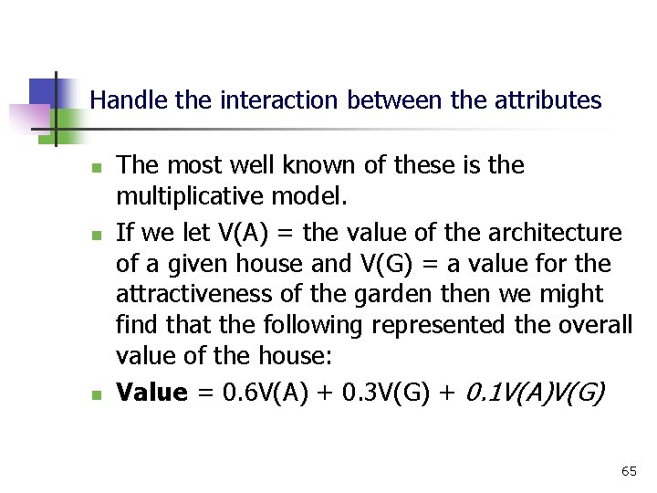
Handle the interaction between the attributes n n n The most well known of these is the multiplicative model. If we let V(A) = the value of the architecture of a given house and V(G) = a value for the attractiveness of the garden then we might find that the following represented the overall value of the house: Value = 0. 6 V(A) + 0. 3 V(G) + 0. 1 V(A)V(G) 65

Conflicts between intuitive and analytic results n n n The larger the problem, the less reliable holistic judgments may be. Discrepancies between holistic and analytic results may result when the axioms are not acceptable to the decision maker. Any conflict between holistic and analytic rankings should be examined, since it may suggest that an important element of the problem has not been captured by the analysis. 66

Variants of SMART n Value focused thinking, but not alternative focused thinking' 67

SMARTER n n n SMARTER differs from SMART in two ways. First, value functions are normally assumed to be linear. The second difference between SMART and SMARTER relates to the elicitation of the swing weights. 68

n n In SMARTER we still have to compare swings, but the process is made easier by simply asking the decision maker to rank the swings in order of importance, rather than asking for a number to represent the relative importance. SMARTER then uses what are known as ‘rank order centroid’, or ROC, weights to convert these rankings into a set of approximate weights. 69

n Table 3. 3 shows the ROC weights for decision problems involving up to seven attributes 70