Chapter 3 Decision Analysis Prepared by Lee Revere
Chapter 3 Decision Analysis Prepared by Lee Revere and John Large To accompany Quantitative Analysis for Management, 9 e by Render/Stair/Hanna 3 -1 1
Learning Objectives Students will be able to: 1. List the steps of the decision-making process. 2. Describe the types of decision-making environments. 3. Make decisions under uncertainty. 4. Use probability values to make decisions under risk. 5. Develop accurate and useful decision trees. 6. Revise probabilities using Bayesian analysis. 7. Use computers to solve basic decisionmaking problems. 8. Understand the importance and use of utility theory in decision theory. To accompany Quantitative Analysis for Management, 9 e by Render/Stair/Hanna 3 -2 2

Chapter Outline 3. 1 3. 2 3. 3 3. 4 3. 5 3. 6 3. 7 3. 8 Introduction The Six Steps in Decision Theory Types of Decision-Making Environments Decision Making under Uncertainty Decision Making under Risk Decision Trees How Probability Values Are Estimated by Bayesian Analysis Utility Theory To accompany Quantitative Analysis for Management, 9 e by Render/Stair/Hanna 3 -3 3
Introduction § Decision theory is an analytical and systematic way to tackle problems. § A good decision is based on logic. To accompany Quantitative Analysis for Management, 9 e by Render/Stair/Hanna 3 -4 4
The Six Steps in Decision Theory 1. 2. 3. 4. Clearly define the problem at hand. List the possible alternatives. Identify the possible outcomes. List the payoff or profit of each combination of alternatives and outcomes. 5. Select one of the mathematical decision theory models. 6. Apply the model and make your decision. To accompany Quantitative Analysis for Management, 9 e by Render/Stair/Hanna 3 -5 5
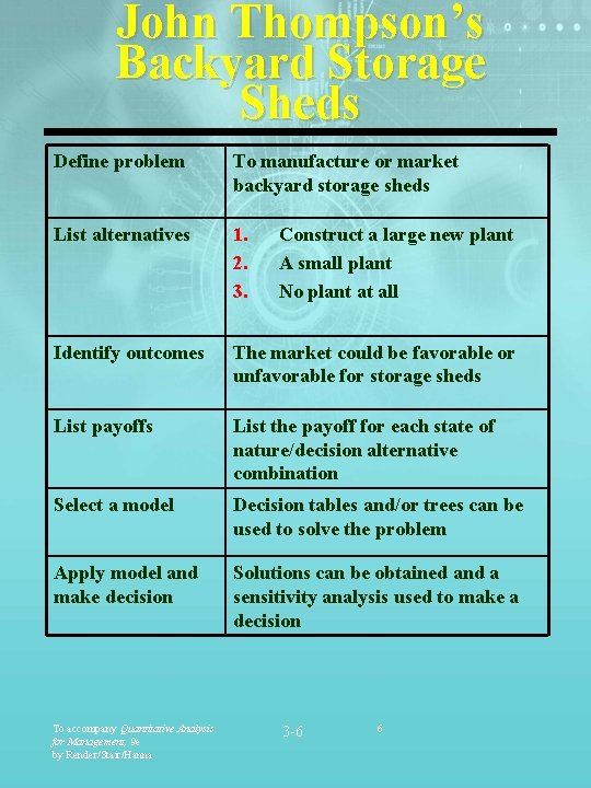
John Thompson’s Backyard Storage Sheds Define problem To manufacture or market backyard storage sheds List alternatives 1. 2. 3. Identify outcomes The market could be favorable or unfavorable for storage sheds List payoffs List the payoff for each state of nature/decision alternative combination Select a model Decision tables and/or trees can be used to solve the problem Apply model and make decision Solutions can be obtained and a sensitivity analysis used to make a decision To accompany Quantitative Analysis for Management, 9 e by Render/Stair/Hanna Construct a large new plant A small plant No plant at all 3 -6 6
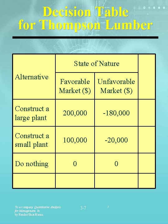
Decision Table for Thompson Lumber State of Nature Alternative Favorable Unfavorable Market ($) Construct a large plant 200, 000 -180, 000 Construct a small plant 100, 000 -20, 000 Do nothing 0 0 To accompany Quantitative Analysis for Management, 9 e by Render/Stair/Hanna 3 -7 7
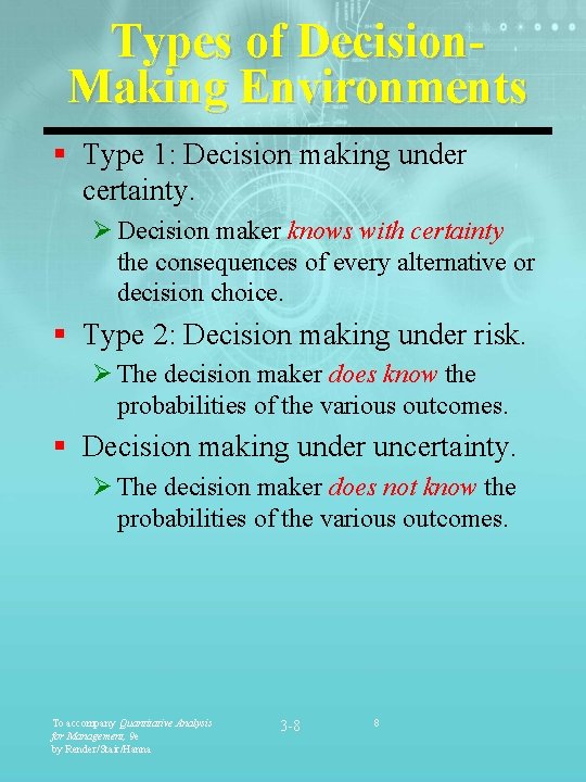
Types of Decision. Making Environments § Type 1: Decision making under certainty. Ø Decision maker knows with certainty the consequences of every alternative or decision choice. § Type 2: Decision making under risk. Ø The decision maker does know the probabilities of the various outcomes. § Decision making under uncertainty. Ø The decision maker does not know the probabilities of the various outcomes. To accompany Quantitative Analysis for Management, 9 e by Render/Stair/Hanna 3 -8 8
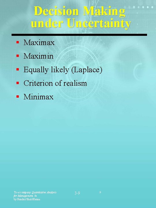
Decision Making under Uncertainty § Maximax § Maximin § Equally likely (Laplace) § Criterion of realism § Minimax To accompany Quantitative Analysis for Management, 9 e by Render/Stair/Hanna 3 -9 9
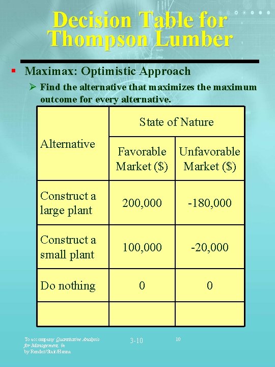
Decision Table for Thompson Lumber § Maximax: Optimistic Approach Ø Find the alternative that maximizes the maximum outcome for every alternative. State of Nature Alternative Favorable Unfavorable Market ($) Construct a large plant 200, 000 -180, 000 Construct a small plant 100, 000 -20, 000 Do nothing 0 0 To accompany Quantitative Analysis for Management, 9 e by Render/Stair/Hanna 3 -10 10
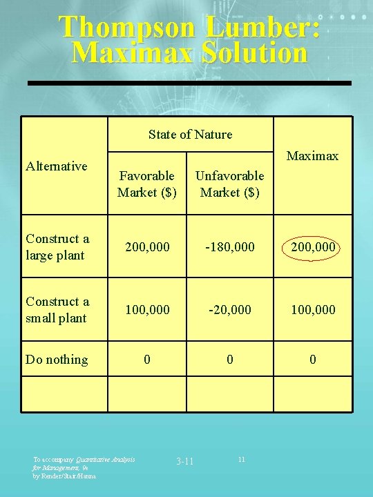
Thompson Lumber: Maximax Solution State of Nature Alternative Maximax Favorable Market ($) Unfavorable Market ($) Construct a large plant 200, 000 -180, 000 200, 000 Construct a small plant 100, 000 -20, 000 100, 000 Do nothing 0 0 0 To accompany Quantitative Analysis for Management, 9 e by Render/Stair/Hanna 3 -11 11
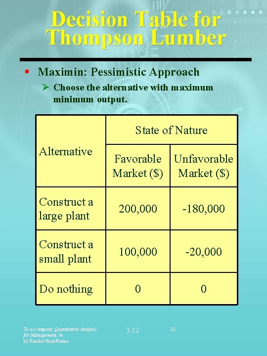
Decision Table for Thompson Lumber § Maximin: Pessimistic Approach Ø Choose the alternative with maximum minimum output. State of Nature Alternative Favorable Unfavorable Market ($) Construct a large plant 200, 000 -180, 000 Construct a small plant 100, 000 -20, 000 Do nothing 0 0 To accompany Quantitative Analysis for Management, 9 e by Render/Stair/Hanna 3 -12 12
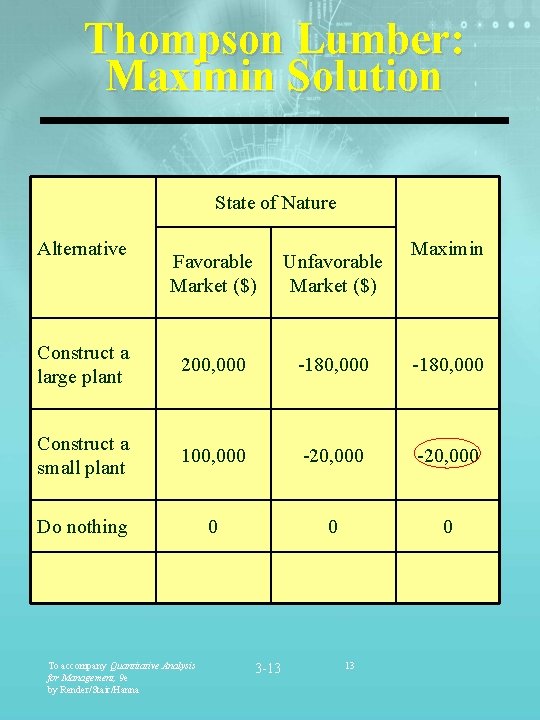
Thompson Lumber: Maximin Solution State of Nature Alternative Maximin Favorable Market ($) Unfavorable Market ($) Construct a large plant 200, 000 -180, 000 Construct a small plant 100, 000 -20, 000 Do nothing 0 0 0 To accompany Quantitative Analysis for Management, 9 e by Render/Stair/Hanna 3 -13 13
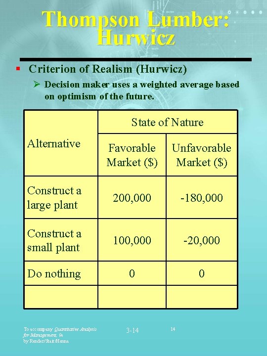
Thompson Lumber: Hurwicz § Criterion of Realism (Hurwicz) Ø Decision maker uses a weighted average based on optimism of the future. State of Nature Alternative Favorable Market ($) Unfavorable Market ($) Construct a large plant 200, 000 -180, 000 Construct a small plant 100, 000 -20, 000 Do nothing 0 0 To accompany Quantitative Analysis for Management, 9 e by Render/Stair/Hanna 3 -14 14
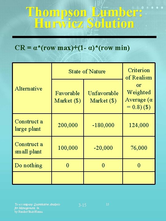
Thompson Lumber: Hurwicz Solution CR = α*(row max)+(1 - α)*(row min) State of Nature Alternative Criterion of Realism or Weighted Average (α = 0. 8) ($) Favorable Market ($) Unfavorable Market ($) Construct a large plant 200, 000 -180, 000 124, 000 Construct a small plant 100, 000 -20, 000 76, 000 Do nothing 0 0 0 To accompany Quantitative Analysis for Management, 9 e by Render/Stair/Hanna 3 -15 15
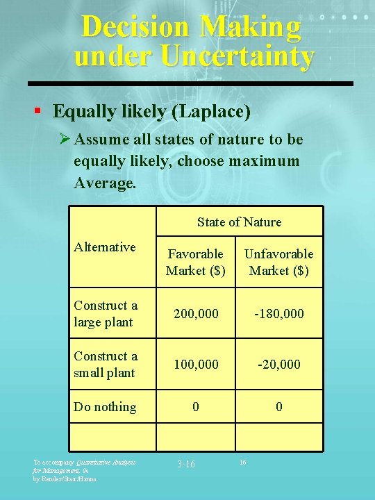
Decision Making under Uncertainty § Equally likely (Laplace) Ø Assume all states of nature to be equally likely, choose maximum Average. State of Nature Alternative Favorable Market ($) Unfavorable Market ($) Construct a large plant 200, 000 -180, 000 Construct a small plant 100, 000 -20, 000 Do nothing 0 0 To accompany Quantitative Analysis for Management, 9 e by Render/Stair/Hanna 3 -16 16
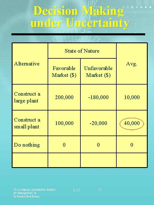
Decision Making under Uncertainty State of Nature Alternative Avg. Favorable Market ($) Unfavorable Market ($) Construct a large plant 200, 000 -180, 000 10, 000 Construct a small plant 100, 000 -20, 000 40, 000 Do nothing 0 0 0 To accompany Quantitative Analysis for Management, 9 e by Render/Stair/Hanna 3 -17 17
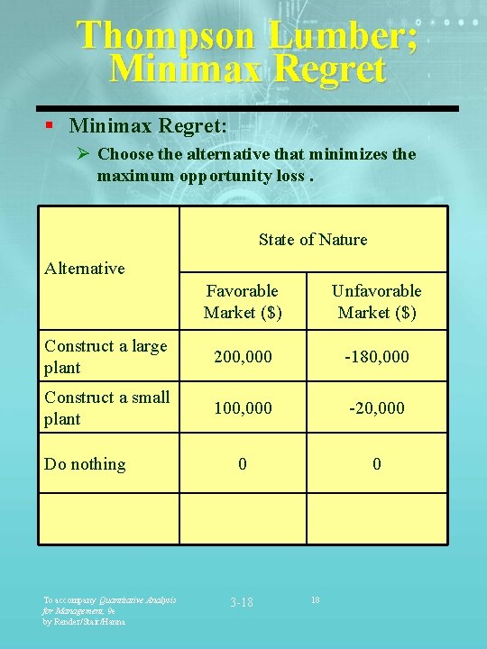
Thompson Lumber; Minimax Regret § Minimax Regret: Ø Choose the alternative that minimizes the maximum opportunity loss. State of Nature Alternative Favorable Market ($) Unfavorable Market ($) Construct a large plant 200, 000 -180, 000 Construct a small plant 100, 000 -20, 000 0 0 Do nothing To accompany Quantitative Analysis for Management, 9 e by Render/Stair/Hanna 3 -18 18
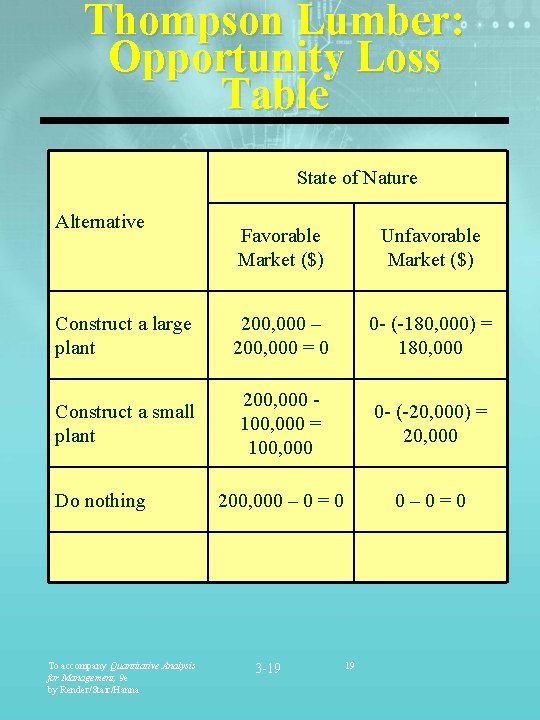
Thompson Lumber: Opportunity Loss Table State of Nature Alternative Favorable Market ($) Unfavorable Market ($) Construct a large plant 200, 000 – 200, 000 = 0 0 - (-180, 000) = 180, 000 Construct a small plant 200, 000 100, 000 = 100, 000 0 - (-20, 000) = 20, 000 200, 000 – 0 = 0 0– 0=0 Do nothing To accompany Quantitative Analysis for Management, 9 e by Render/Stair/Hanna 3 -19 19
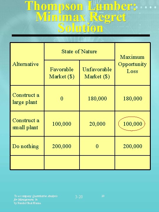
Thompson Lumber: Minimax Regret Solution State of Nature Alternative Maximum Opportunity Loss Favorable Market ($) Unfavorable Market ($) Construct a large plant 0 180, 000 Construct a small plant 100, 000 20, 000 100, 000 Do nothing 200, 000 0 200, 000 To accompany Quantitative Analysis for Management, 9 e by Render/Stair/Hanna 3 -20 20
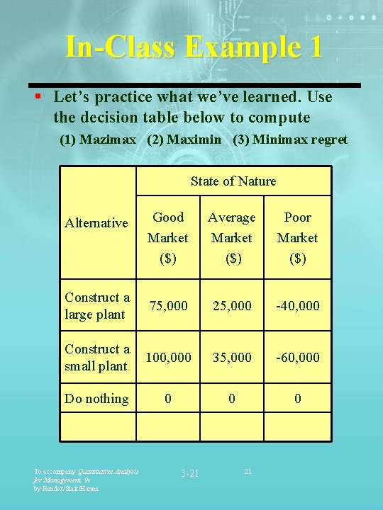
In-Class Example 1 § Let’s practice what we’ve learned. Use the decision table below to compute (1) Mazimax (2) Maximin (3) Minimax regret State of Nature Good Market ($) Average Market ($) Poor Market ($) Construct a large plant 75, 000 25, 000 -40, 000 Construct a small plant 100, 000 35, 000 -60, 000 Do nothing 0 0 0 Alternative To accompany Quantitative Analysis for Management, 9 e by Render/Stair/Hanna 3 -21 21
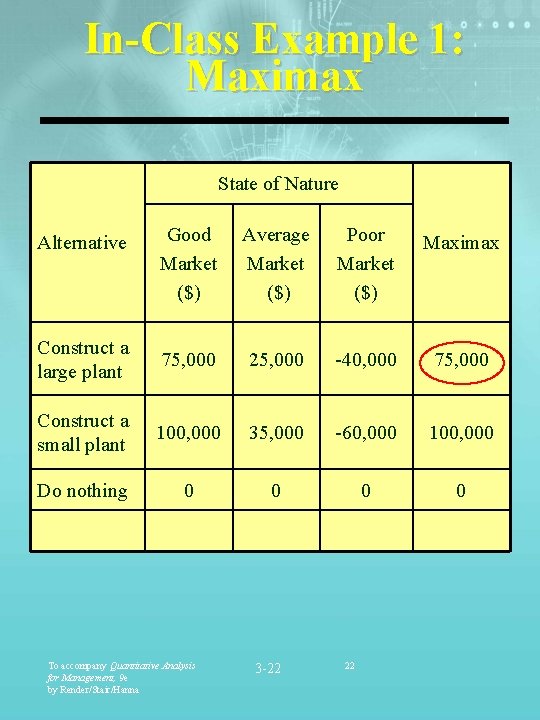
In-Class Example 1: Maximax State of Nature Good Market ($) Average Market ($) Poor Market ($) Maximax Construct a large plant 75, 000 25, 000 -40, 000 75, 000 Construct a small plant 100, 000 35, 000 -60, 000 100, 000 Do nothing 0 0 To accompany Quantitative Analysis for Management, 9 e by Render/Stair/Hanna 3 -22 Alternative 22
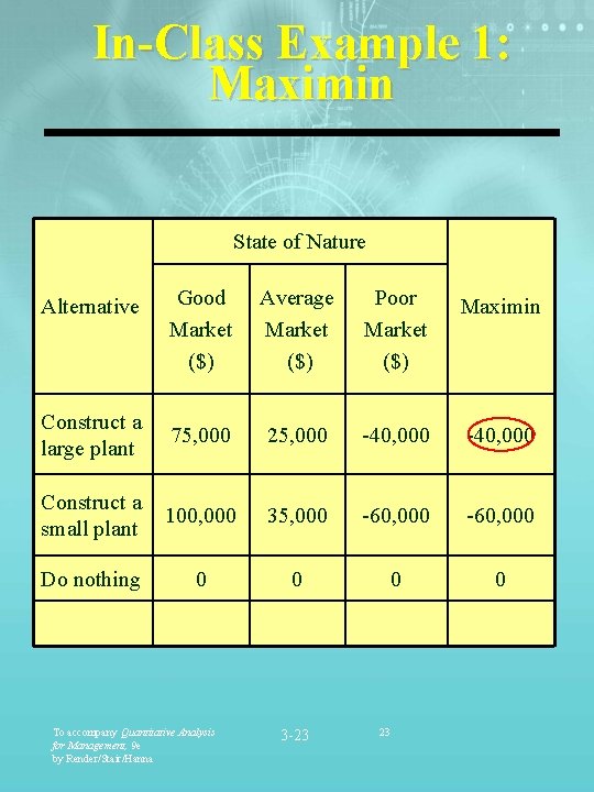
In-Class Example 1: Maximin State of Nature Good Market ($) Average Market ($) Poor Market ($) Maximin Construct a large plant 75, 000 25, 000 -40, 000 Construct a small plant 100, 000 35, 000 -60, 000 Do nothing 0 0 Alternative To accompany Quantitative Analysis for Management, 9 e by Render/Stair/Hanna 3 -23 23
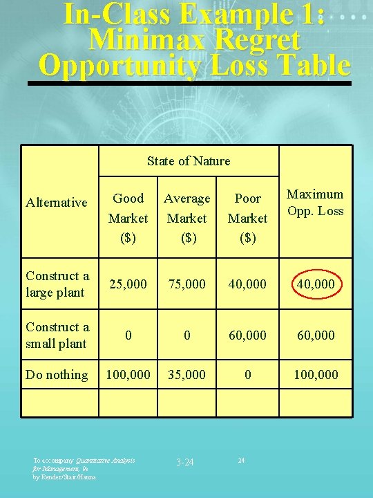
In-Class Example 1: Minimax Regret Opportunity Loss Table State of Nature Good Market ($) Average Market ($) Poor Market ($) Maximum Opp. Loss Construct a large plant 25, 000 75, 000 40, 000 Construct a small plant 0 0 60, 000 Do nothing 100, 000 35, 000 0 100, 000 Alternative To accompany Quantitative Analysis for Management, 9 e by Render/Stair/Hanna 3 -24 24
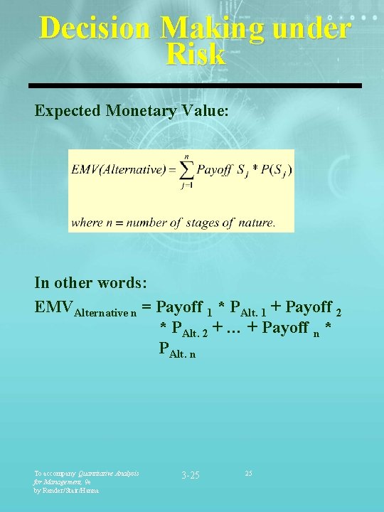
Decision Making under Risk Expected Monetary Value: In other words: EMVAlternative n = Payoff 1 * PAlt. 1 + Payoff 2 * PAlt. 2 + … + Payoff n * PAlt. n To accompany Quantitative Analysis for Management, 9 e by Render/Stair/Hanna 3 -25 25
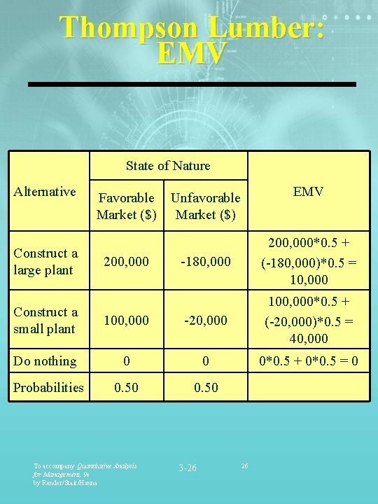
Thompson Lumber: EMV State of Nature Alternative Construct a large plant Favorable Market ($) 200, 000 EMV Unfavorable Market ($) -180, 000 200, 000*0. 5 + (-180, 000)*0. 5 = 10, 000 Construct a small plant 100, 000 -20, 000 100, 000*0. 5 + (-20, 000)*0. 5 = 40, 000 Do nothing 0 0 0*0. 5 + 0*0. 5 = 0 Probabilities 0. 50 To accompany Quantitative Analysis for Management, 9 e by Render/Stair/Hanna 3 -26 26
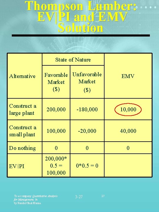
Thompson Lumber: EV|PI and EMV Solution State of Nature Alternative Favorable Unfavorable Market ($) EMV Construct a large plant 200, 000 -180, 000 10, 000 Construct a small plant 100, 000 -20, 000 40, 000 Do nothing 0 0 0 200, 000* 0. 5 = 100, 000 0*0. 5 = 0 EV ׀ PI To accompany Quantitative Analysis for Management, 9 e by Render/Stair/Hanna 3 -27 27
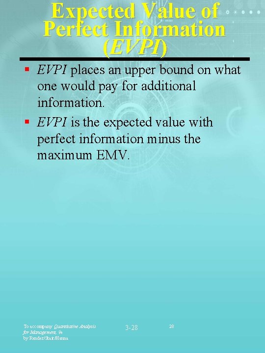
Expected Value of Perfect Information (EVPI) § EVPI places an upper bound on what one would pay for additional information. § EVPI is the expected value with perfect information minus the maximum EMV. To accompany Quantitative Analysis for Management, 9 e by Render/Stair/Hanna 3 -28 28
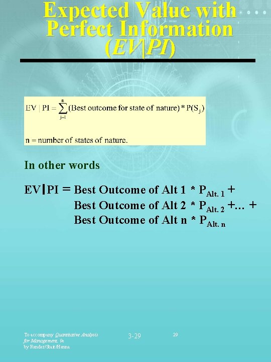
Expected Value with Perfect Information (EV|PI) In other words EV ׀ PI = Best Outcome of Alt 1 * PAlt. 1 + Best Outcome of Alt 2 * PAlt. 2 +… + Best Outcome of Alt n * PAlt. n To accompany Quantitative Analysis for Management, 9 e by Render/Stair/Hanna 3 -29 29
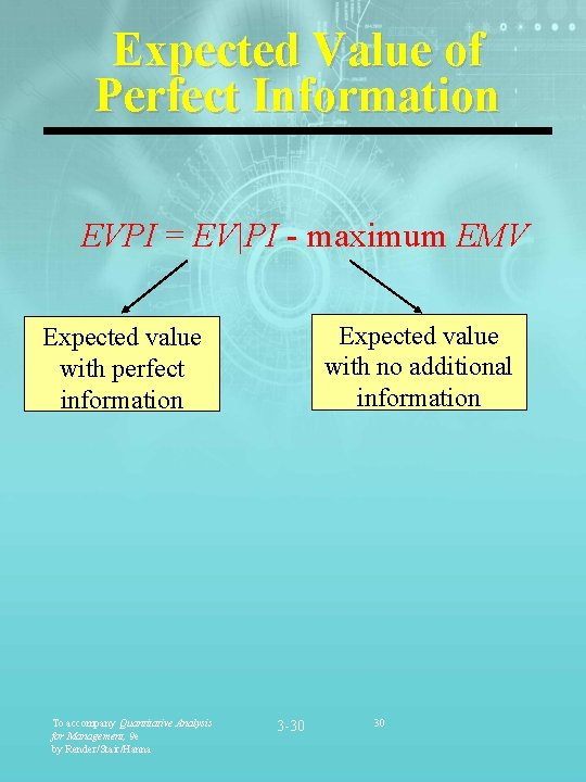
Expected Value of Perfect Information EVPI = EV|PI - maximum EMV Expected value with no additional information Expected value with perfect information To accompany Quantitative Analysis for Management, 9 e by Render/Stair/Hanna 3 -30 30
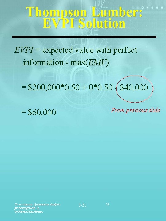
Thompson Lumber: EVPI Solution EVPI = expected value with perfect information - max(EMV) EMV = $200, 000*0. 50 + 0*0. 50 - $40, 000 From previous slide = $60, 000 To accompany Quantitative Analysis for Management, 9 e by Render/Stair/Hanna 3 -31 31
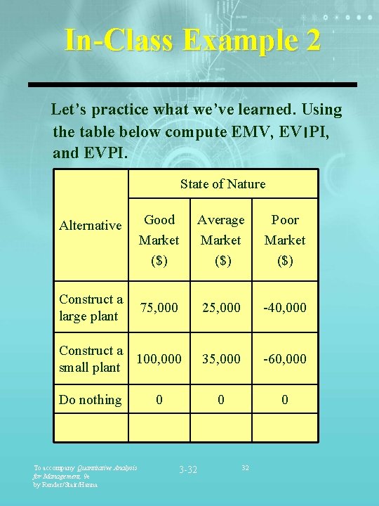
In-Class Example 2 Let’s practice what we’ve learned. Using the table below compute EMV, EV ׀ PI, and EVPI. State of Nature Good Market ($) Average Market ($) Poor Market ($) 75, 000 25, 000 -40, 000 Construct a 100, 000 small plant 35, 000 -60, 000 0 0 Alternative Construct a large plant Do nothing To accompany Quantitative Analysis for Management, 9 e by Render/Stair/Hanna 0 3 -32 32
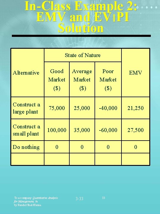
In-Class Example 2: EMV and EV ׀ PI Solution State of Nature Good Market ($) Average Market ($) Poor Market ($) EMV Construct a large plant 75, 000 25, 000 -40, 000 21, 250 Construct a small plant 100, 000 35, 000 -60, 000 27, 500 Do nothing 0 0 To accompany Quantitative Analysis for Management, 9 e by Render/Stair/Hanna 3 -33 Alternative 33
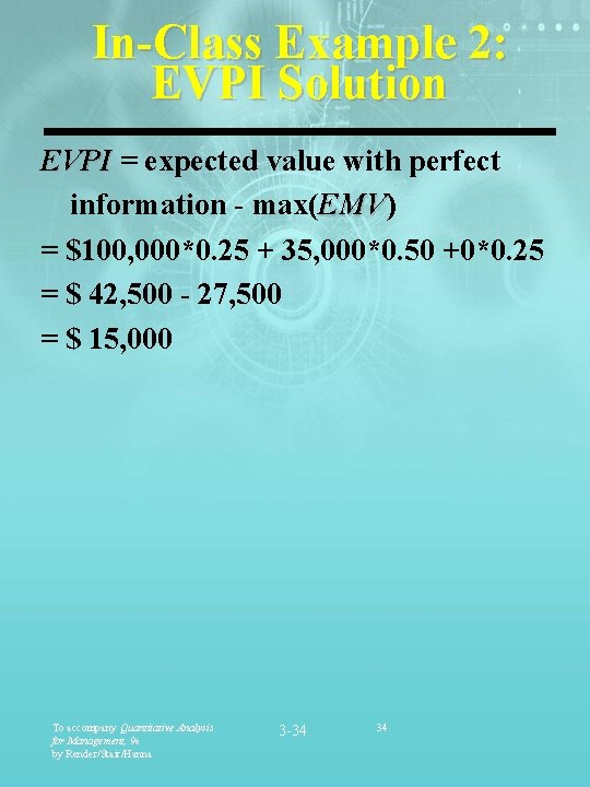
In-Class Example 2: EVPI Solution EVPI = expected value with perfect information - max(EMV) EMV = $100, 000*0. 25 + 35, 000*0. 50 +0*0. 25 = $ 42, 500 - 27, 500 = $ 15, 000 To accompany Quantitative Analysis for Management, 9 e by Render/Stair/Hanna 3 -34 34

Expected Opportunity Loss § EOL is the cost of not picking the best solution. EOL = Expected Regret To accompany Quantitative Analysis for Management, 9 e by Render/Stair/Hanna 3 -35 35
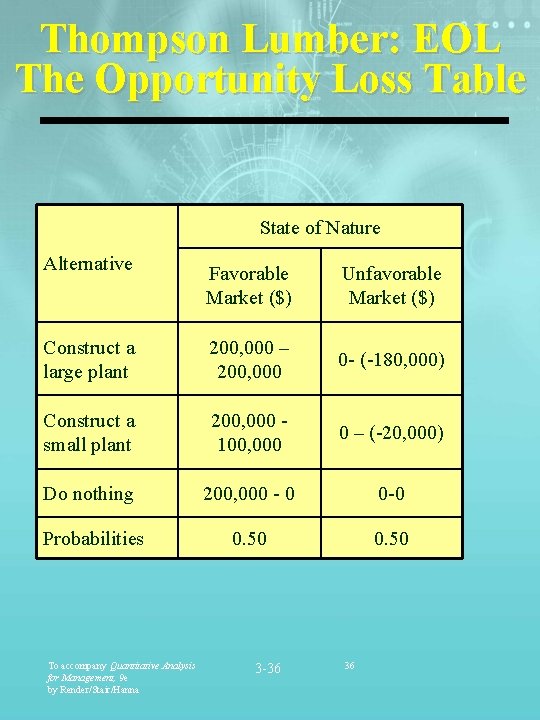
Thompson Lumber: EOL The Opportunity Loss Table State of Nature Alternative Favorable Market ($) Unfavorable Market ($) Construct a large plant 200, 000 – 200, 000 0 - (-180, 000) Construct a small plant 200, 000 100, 000 0 – (-20, 000) Do nothing 200, 000 - 0 0 -0 Probabilities 0. 50 To accompany Quantitative Analysis for Management, 9 e by Render/Stair/Hanna 3 -36 36
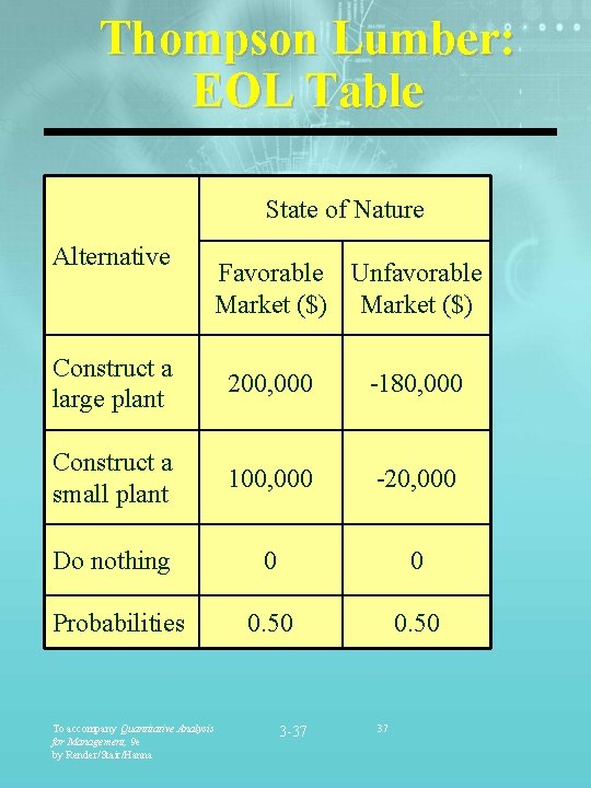
Thompson Lumber: EOL Table State of Nature Alternative Favorable Unfavorable Market ($) Construct a large plant 200, 000 -180, 000 Construct a small plant 100, 000 -20, 000 Do nothing 0 0 Probabilities 0. 50 To accompany Quantitative Analysis for Management, 9 e by Render/Stair/Hanna 3 -37 37
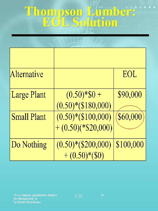
Thompson Lumber: EOL Solution To accompany Quantitative Analysis for Management, 9 e by Render/Stair/Hanna 3 -38 38
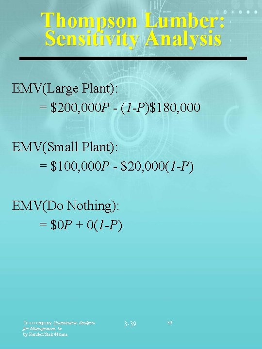
Thompson Lumber: Sensitivity Analysis EMV(Large Plant): = $200, 000 P - (1 -P)$180, 000 EMV(Small Plant): = $100, 000 P - $20, 000(1 -P) EMV(Do Nothing): = $0 P + 0(1 -P) To accompany Quantitative Analysis for Management, 9 e by Render/Stair/Hanna 3 -39 39
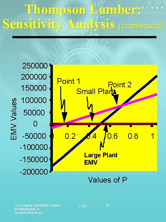
Thompson Lumber: Sensitivity Analysis (continued) EMV Values 250000 200000 150000 Point 1 Point 2 Small Plant 100000 50000 0 -100000 -150000 0. 2 0. 4 Large Plant EMV -200000 To accompany Quantitative Analysis for Management, 9 e by Render/Stair/Hanna 0. 6 Values of P 3 -40 40 0. 8 1
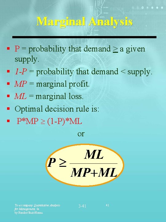
Marginal Analysis § P = probability that demand > a given supply. § 1 -P = probability that demand < supply. § MP = marginal profit. § ML = marginal loss. § Optimal decision rule is: § P*MP (1 -P)*ML or To accompany Quantitative Analysis for Management, 9 e by Render/Stair/Hanna 3 -41 41
Marginal Analysis Discrete Distributions Steps using Discrete Distributions: § Determine the value for P. § Construct a probability table and add a cumulative probability column. § Keep ordering inventory as long as the probability of selling at least one additional unit is greater than P. To accompany Quantitative Analysis for Management, 9 e by Render/Stair/Hanna 3 -42 42
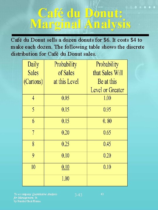
Café du Donut: Marginal Analysis Café du Donut sells a dozen donuts for $6. It costs $4 to make each dozen. The following table shows the discrete distribution for Café du Donut sales. To accompany Quantitative Analysis for Management, 9 e by Render/Stair/Hanna 3 -43 43
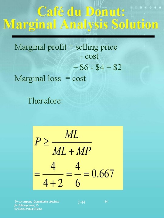
Café du Donut: Marginal Analysis Solution Marginal profit = selling price - cost = $6 - $4 = $2 Marginal loss = cost Therefore: To accompany Quantitative Analysis for Management, 9 e by Render/Stair/Hanna 3 -44 44
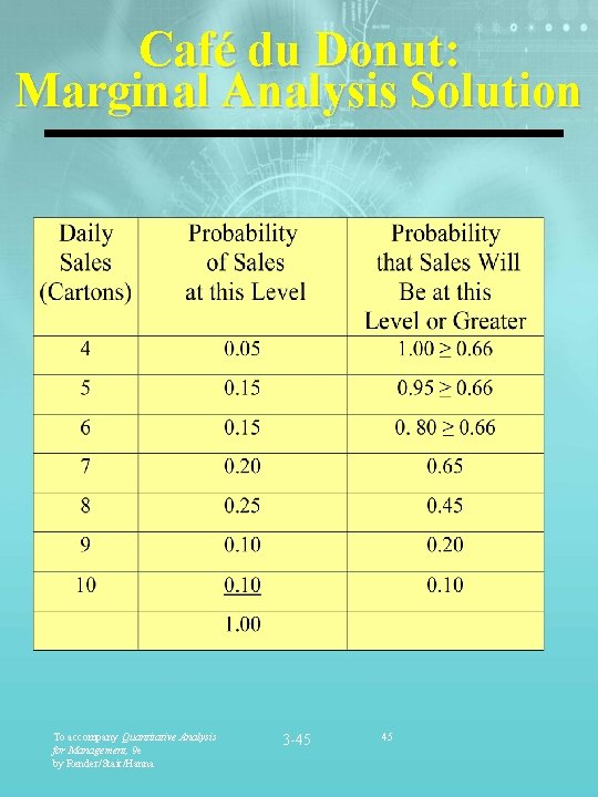
Café du Donut: Marginal Analysis Solution To accompany Quantitative Analysis for Management, 9 e by Render/Stair/Hanna 3 -45 45
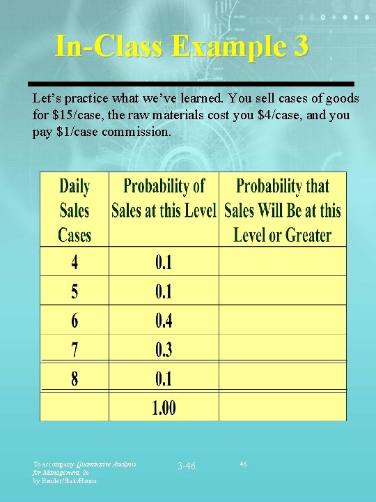
In-Class Example 3 Let’s practice what we’ve learned. You sell cases of goods for $15/case, the raw materials cost you $4/case, and you pay $1/case commission. To accompany Quantitative Analysis for Management, 9 e by Render/Stair/Hanna 3 -46 46
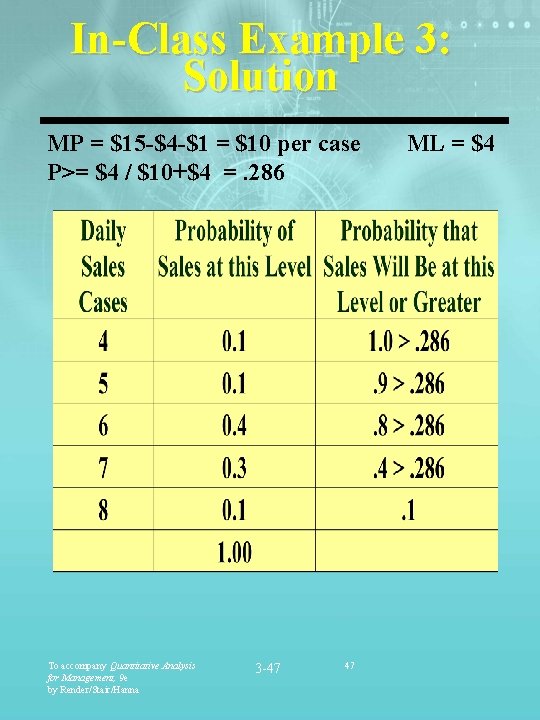
In-Class Example 3: Solution MP = $15 -$4 -$1 = $10 per case P>= $4 / $10+$4 =. 286 To accompany Quantitative Analysis for Management, 9 e by Render/Stair/Hanna 3 -47 47 ML = $4
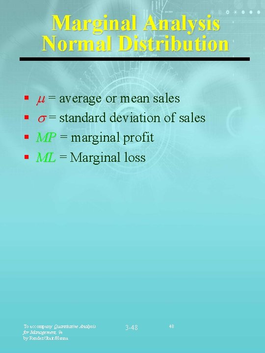
Marginal Analysis Normal Distribution § § = average or mean sales = standard deviation of sales MP = marginal profit ML = Marginal loss To accompany Quantitative Analysis for Management, 9 e by Render/Stair/Hanna 3 -48 48
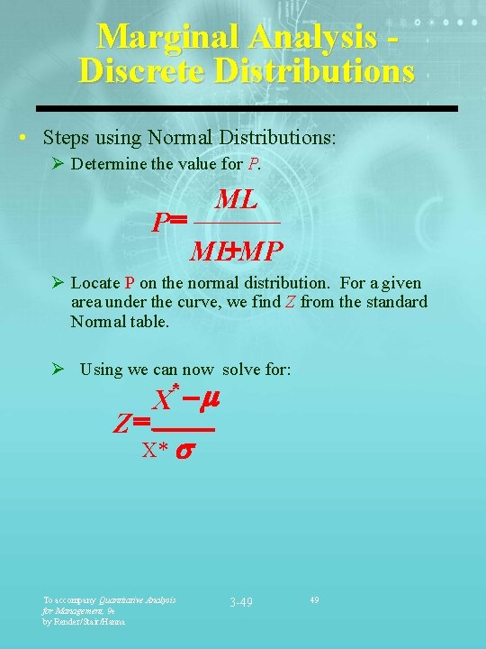
Marginal Analysis Discrete Distributions • Steps using Normal Distributions: Ø Determine the value for P. P= ML ML+MP Ø Locate P on the normal distribution. For a given area under the curve, we find Z from the standard Normal table. Ø Using we can now solve for: * Z= X -m X* s To accompany Quantitative Analysis for Management, 9 e by Render/Stair/Hanna 3 -49 49
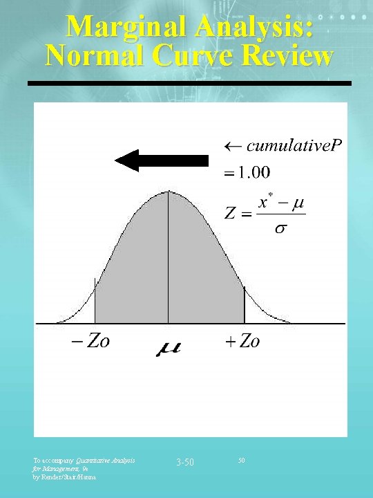
Marginal Analysis: Normal Curve Review To accompany Quantitative Analysis for Management, 9 e by Render/Stair/Hanna 3 -50 50
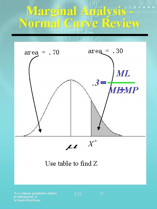
Marginal Analysis Normal Curve Review area =. 30 area =. 70 . 3 = Use table to find Z To accompany Quantitative Analysis for Management, 9 e by Render/Stair/Hanna 3 -51 51 ML ML+MP
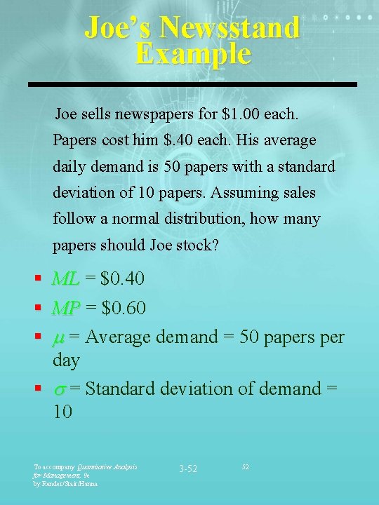
Joe’s Newsstand Example Joe sells newspapers for $1. 00 each. Papers cost him $. 40 each. His average daily demand is 50 papers with a standard deviation of 10 papers. Assuming sales follow a normal distribution, how many papers should Joe stock? § ML = $0. 40 § MP = $0. 60 § = Average demand = 50 papers per day § = Standard deviation of demand = 10 To accompany Quantitative Analysis for Management, 9 e by Render/Stair/Hanna 3 -52 52
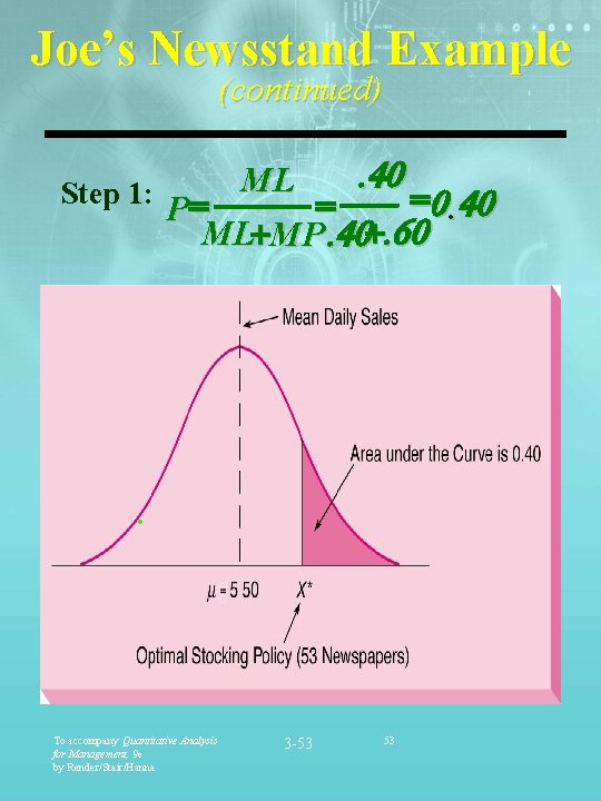
Joe’s Newsstand Example (continued) . 40 ML Step 1: = =0. 40 = P ML+MP. 40+. 60 . To accompany Quantitative Analysis for Management, 9 e by Render/Stair/Hanna 3 -53 53
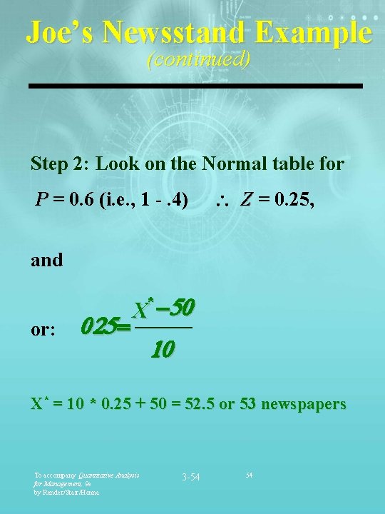
Joe’s Newsstand Example (continued) Step 2: Look on the Normal table for P = 0. 6 (i. e. , 1 -. 4) Z = 0. 25, and or: 0 25 = X -50 * 10 X* = 10 * 0. 25 + 50 = 52. 5 or 53 newspapers To accompany Quantitative Analysis for Management, 9 e by Render/Stair/Hanna 3 -54 54
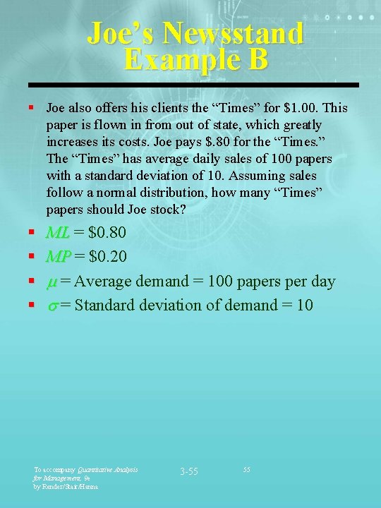
Joe’s Newsstand Example B § Joe also offers his clients the “Times” for $1. 00. This paper is flown in from out of state, which greatly increases its costs. Joe pays $. 80 for the “Times. ” The “Times” has average daily sales of 100 papers with a standard deviation of 10. Assuming sales follow a normal distribution, how many “Times” papers should Joe stock? § § ML = $0. 80 MP = $0. 20 = Average demand = 100 papers per day = Standard deviation of demand = 10 To accompany Quantitative Analysis for Management, 9 e by Render/Stair/Hanna 3 -55 55
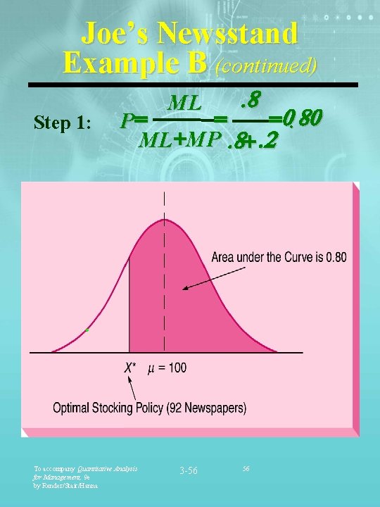
Joe’s Newsstand Example B (continued) Step 1: . 8 ML = =0. 80 P= ML +MP. 8+. 2 . To accompany Quantitative Analysis for Management, 9 e by Render/Stair/Hanna 3 -56 56
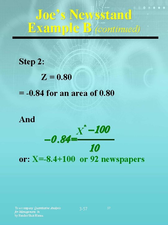
Joe’s Newsstand Example B (continued) Step 2: Z = 0. 80 = -0. 84 for an area of 0. 80 And X -100 -0. 84 = * 10 or: X=-8. 4+100 or 92 newspapers To accompany Quantitative Analysis for Management, 9 e by Render/Stair/Hanna 3 -57 57
Decision Making with Uncertainty: Using the Decision Trees Decision trees enable one to look at decisions: § With many alternatives and states of nature, § which must be made in sequence. To accompany Quantitative Analysis for Management, 9 e by Render/Stair/Hanna 3 -58 58
Five Steps to Decision Tree Analysis 1. Define the problem. 2. Structure or draw the decision tree. 3. Assign probabilities to the states of nature. 4. Estimate payoffs for each possible combination of alternatives and states of nature. 5. Solve the problem by computing expected monetary values (EMVs) for each state of nature node. To accompany Quantitative Analysis for Management, 9 e by Render/Stair/Hanna 3 -59 59
Structure of Decision Trees A graphical representation where: § A decision node from which one of several alternatives may be chosen. § A state-of-nature node out of which one state of nature will occur. To accompany Quantitative Analysis for Management, 9 e by Render/Stair/Hanna 3 -60 60
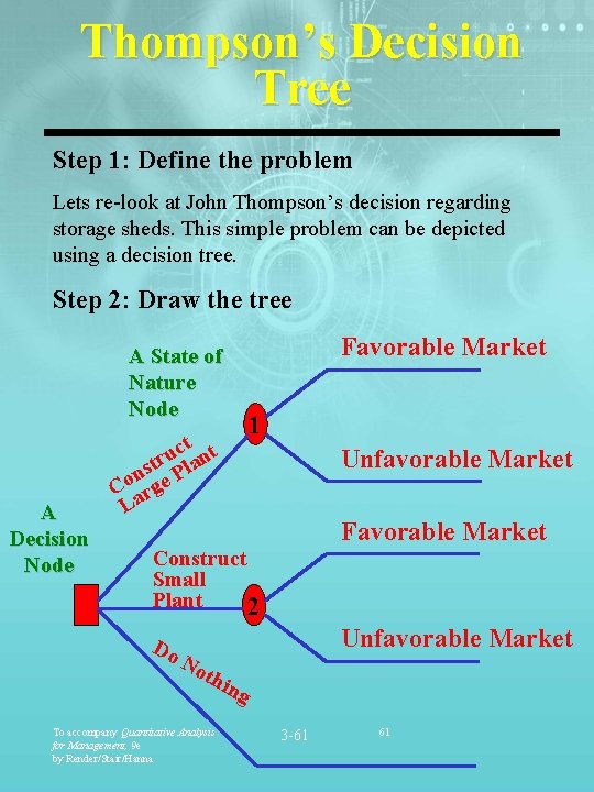
Thompson’s Decision Tree Step 1: Define the problem Lets re-look at John Thompson’s decision regarding storage sheds. This simple problem can be depicted using a decision tree. Step 2: Draw the tree Favorable Market A State of Nature Node A Decision Node 1 ct nt u str Pla n Co arge L Unfavorable Market Favorable Market Construct Small Plant 2 Do Unfavorable Market No thi n To accompany Quantitative Analysis for Management, 9 e by Render/Stair/Hanna g 3 -61 61
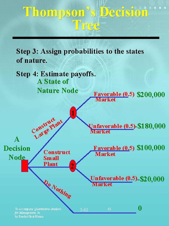
Thompson’s Decision Tree Step 3: Assign probabilities to the states of nature. Step 4: Estimate payoffs. A State of Nature Node Favorable (0. 5) Market A Decision Node 1 ct nt u str Pla n Co arge L Unfavorable (0. 5)-$180, 000 Market Favorable (0. 5) Market Construct Small Plant 2 Do $200, 000 $100, 000 Unfavorable (0. 5)-$20, 000 Market No thi ng To accompany Quantitative Analysis for Management, 9 e by Render/Stair/Hanna 3 -62 62 0
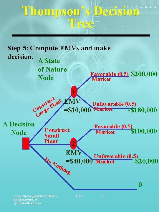
Thompson’s Decision Tree Step 5: Compute EMVs and make decision. A State of Nature Favorable (0. 5) $200, 000 Node Market 1 ct nt EMV u Unfavorable (0. 5) str Pla n =$10, 000 Market -$180, 000 Co arge L A Decision Node Favorable (0. 5) $100, 000 Market Construct Small Plant Do No thi 2 EMV Unfavorable (0. 5) -$20, 000 =$40, 000 Market ng 0 To accompany Quantitative Analysis for Management, 9 e by Render/Stair/Hanna 3 -63 63
Thompson’s Decision: A More Complex Problem § John Thompson has the opportunity of obtaining a market survey that will give additional information on the probable state of nature. Results of the market survey will likely indicate there is a percent change of a favorable market. Historical data show market surveys accurately predict favorable markets 78 % of the time. Thus P(Fav. Mkt / Fav. Survey Results) =. 78 § Likewise, if the market survey predicts an unfavorable market, there is a 13 % chance of its occurring. P(Unfav. Mkt / Unfav. Survey Results) =. 13 § Now that we have redefined the problem (Step 1), let’s use this additional data and redraw Thompson’s decision tree (Step 2). To accompany Quantitative Analysis for Management, 9 e by Render/Stair/Hanna 3 -64 64
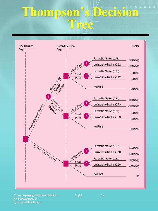
Thompson’s Decision Tree To accompany Quantitative Analysis for Management, 9 e by Render/Stair/Hanna 3 -65 65
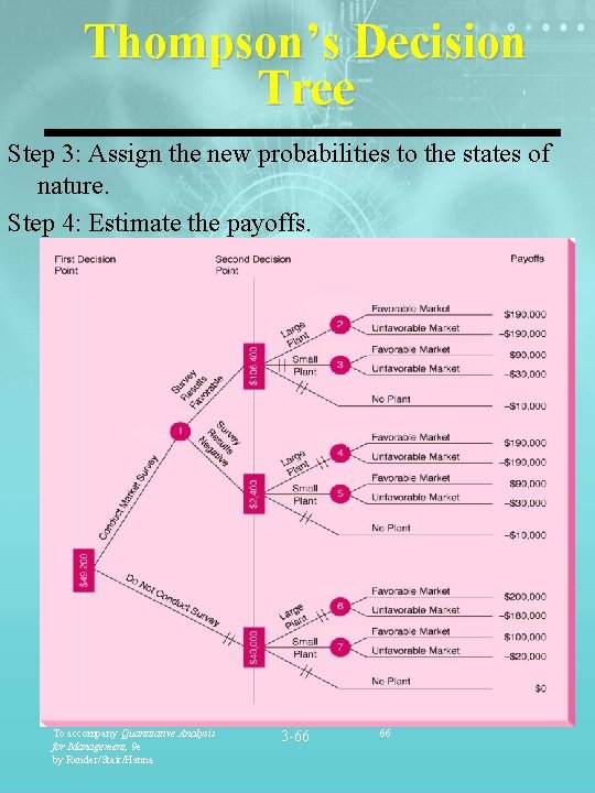
Thompson’s Decision Tree Step 3: Assign the new probabilities to the states of nature. Step 4: Estimate the payoffs. To accompany Quantitative Analysis for Management, 9 e by Render/Stair/Hanna 3 -66 66
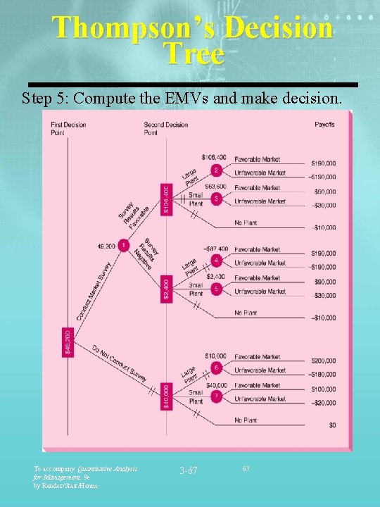
Thompson’s Decision Tree Step 5: Compute the EMVs and make decision. To accompany Quantitative Analysis for Management, 9 e by Render/Stair/Hanna 3 -67 67
John Thompson Dilemma John Thompson is not sure how much value to place on market survey. He wants to determine the monetary worth of the survey. John Thompson is also interested in how sensitive his decision is to changes in the market survey results. What should he do? §Expected Value of Sample Information §Sensitivity Analysis To accompany Quantitative Analysis for Management, 9 e by Render/Stair/Hanna 3 -68 68
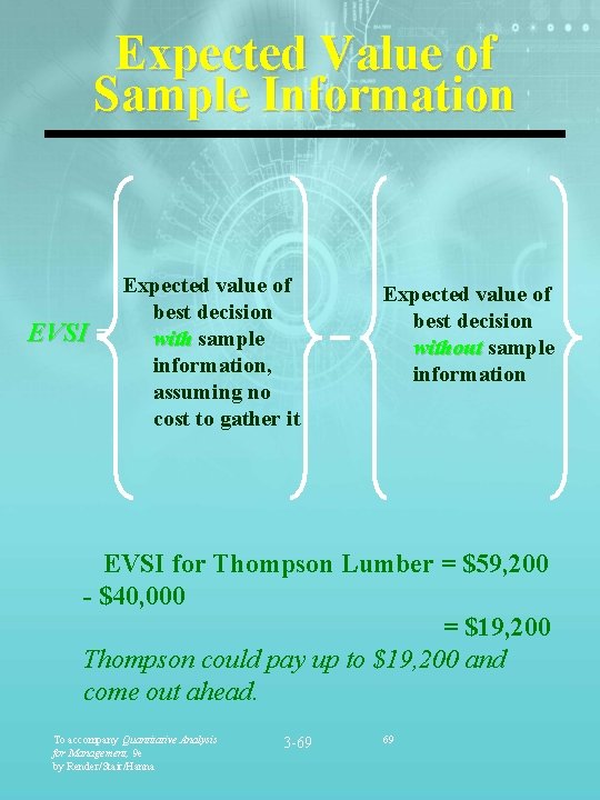
Expected Value of Sample Information EVSI = Expected value of best decision with sample information, assuming no cost to gather it Expected value of best decision without sample information EVSI for Thompson Lumber = $59, 200 - $40, 000 = $19, 200 Thompson could pay up to $19, 200 and come out ahead. To accompany Quantitative Analysis for Management, 9 e by Render/Stair/Hanna 3 -69 69
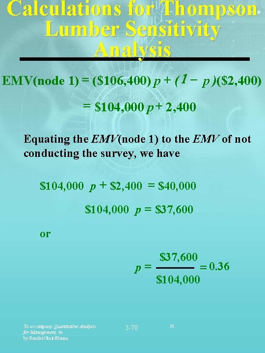
Calculations for Thompson Lumber Sensitivity Analysis EMV(node 1) = ($106, 400) p + ( 1 - p )($2, 400) = $104, 000 p + 2, 400 Equating the EMV(node 1) to the EMV of not EMV conducting the survey, we have $104, 000 p + $2, 400 = $40, 000 $104, 000 p = $37, 600 or p= To accompany Quantitative Analysis for Management, 9 e by Render/Stair/Hanna 3 -70 $37, 600 = 0. 36 $104, 000 70
In-Class Problem 3 Let’s practice what we’ve learned Leo can purchase a historic home for $200, 000 or land in a growing area for $50, 000. There is a 60% chance the economy will grow and a 40% change it will not. If it grows, the historic home will appreciate in value by 15% yielding a $30, 00 profit. If it does not grow, the profit is only $10, 000. If Leo purchases the land he will hold it for 1 year to assess the economic growth. If the economy grew during the first year, there is an 80% chance it will continue to grow. If it did not grow during the first year, there is a 30% chance it will grow in the next 4 years. After a year, if the economy grew, Leo will decide either to build and sell a house or simply sell the land. It will cost Leo $75, 000 to build a house that will sell for a profit of $55, 000 if the economy grows, or $15, 000 if it does not grow. Leo can sell the land for a profit of $15, 000. If, after a year, the economy does not grow, Leo will either develop the land, which will cost $75, 000, or sell the land for a profit of $5, 000. If he develops the land the economy begins to grow, he will make $45, 000. If he develops the land the economy does not grow, he will make $5, 000. To accompany Quantitative Analysis for Management, 9 e by Render/Stair/Hanna 3 -71 71
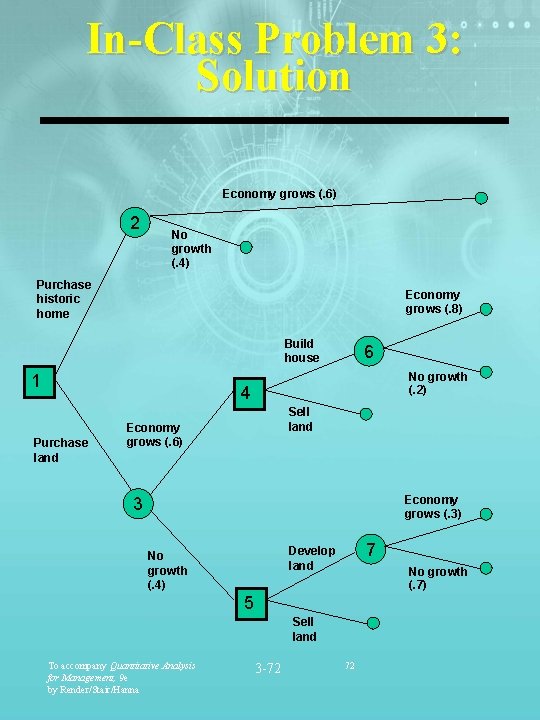
In-Class Problem 3: Solution Economy grows (. 6) 2 No growth (. 4) Purchase historic home Economy grows (. 8) Build house 1 6 No growth (. 2) 4 Purchase land Sell land Economy grows (. 6) Economy grows (. 3) 3 7 Develop land No growth (. 4) No growth (. 7) 5 Sell land To accompany Quantitative Analysis for Management, 9 e by Render/Stair/Hanna 3 -72 72
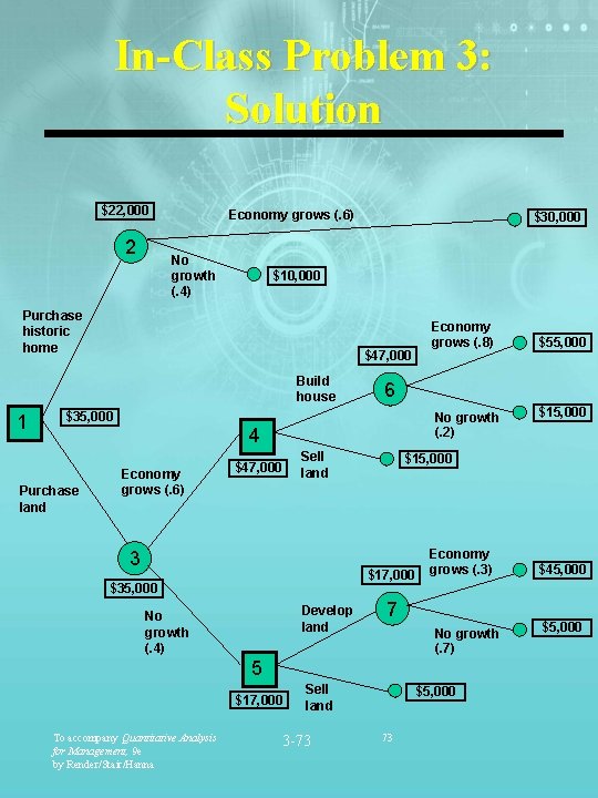
In-Class Problem 3: Solution $22, 000 2 Economy grows (. 6) No growth (. 4) $10, 000 Purchase historic home $47, 000 Build house 1 $35, 000 Purchase land $30, 000 No growth (. 2) $47, 000 Sell land 3 Develop land No growth (. 4) Economy grows (. 3) To accompany Quantitative Analysis for Management, 9 e by Render/Stair/Hanna No growth (. 7) Sell land 3 -73 $45, 000 7 5 $17, 000 $15, 000 $17, 000 $35, 000 $55, 000 6 4 Economy grows (. 6) Economy grows (. 8) $5, 000 73 $5, 000
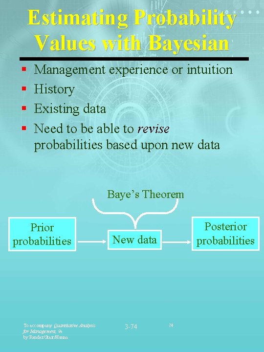
Estimating Probability Values with Bayesian § § Management experience or intuition History Existing data Need to be able to revise probabilities based upon new data Baye’s Theorem Prior probabilities To accompany Quantitative Analysis for Management, 9 e by Render/Stair/Hanna Posterior probabilities New data 3 -74 74
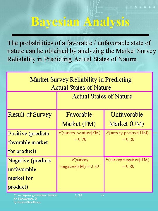
Bayesian Analysis The probabilities of a favorable / unfavorable state of nature can be obtained by analyzing the Market Survey Reliability in Predicting Actual States of Nature Result of Survey Favorable Market (FM) Unfavorable Market (UM) Positive (predicts favorable market for product) P(survey positive|FM) = 0. 70 P(survey positive|UM) = 0. 20 Negative (predicts unfavorable market for product) P(survey negative|FM) = 0. 30 P(survey negative|UM) = 0. 80 To accompany Quantitative Analysis for Management, 9 e by Render/Stair/Hanna 3 -75 75
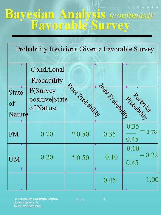
Bayesian Analysis (continued): Favorable Survey Probability Revisions Given a Favorable Survey Conditional Jo 0. 70 * 0. 50 0. 35 UM 0. 20 * 0. 50 0. 10 0. 45 3 -76 r rio ty ste ili Po bab o ty FM To accompany Quantitative Analysis for Management, 9 e by Render/Stair/Hanna Pr y lit ili bi ab ba ro ob Pr r. P io int Pr Probability State P(Survey positive|State of of Nature 76 0. 35 0. 45 0. 10 0. 45 = 0. 78 = 0. 22 1. 00
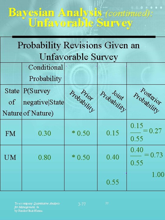
Bayesian Analysis (continued): Unfavorable Survey Probability Revisions Given an Unfavorable Survey Conditional Probability State P(Survey of negative|State Nature of Nature) FM UM 0. 30 0. 80 Pr ob ior ab ili ty Pr * 0. 50 Pr Join ob ab t ilit y 0. 15 0. 40 0. 55 To accompany Quantitative Analysis for Management, 9 e by Render/Stair/Hanna 3 -77 77 Po Pr ste ob rio ab r ilit y 0. 15 0. 55 0. 40 0. 55 = 0. 27 = 0. 73 1. 00
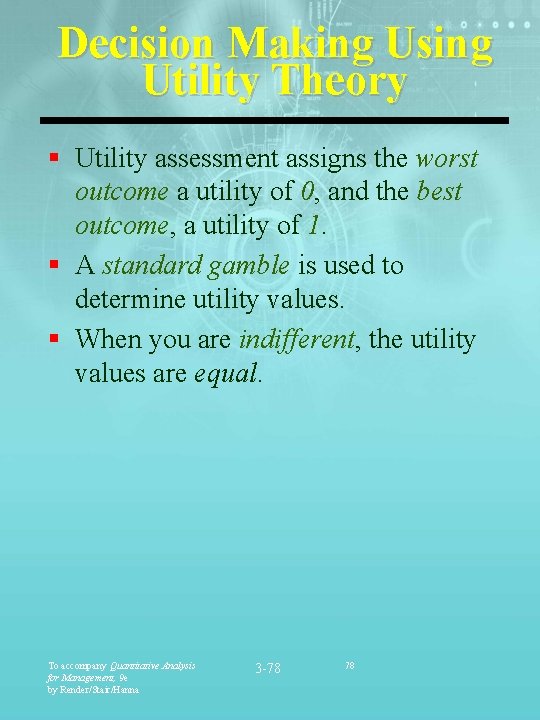
Decision Making Using Utility Theory § Utility assessment assigns the worst outcome a utility of 0, and the best outcome, a utility of 1. § A standard gamble is used to determine utility values. § When you are indifferent, the utility values are equal. To accompany Quantitative Analysis for Management, 9 e by Render/Stair/Hanna 3 -78 78
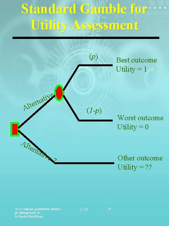
Standard Gamble for Utility Assessment (p) Best outcome Utility = 1 1 e ativ n r e t Al (1 -p) Worst outcome Utility = 0 Alt ern ativ e 2 To accompany Quantitative Analysis for Management, 9 e by Render/Stair/Hanna Other outcome Utility = ? ? 3 -79 79
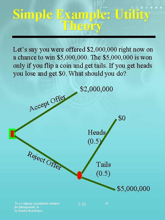
Simple Example: Utility Theory Let’s say you were offered $2, 000 right now on a chance to win $5, 000. The $5, 000 is won only if you flip a coin and get tails. If you get heads you lose and get $0. What should you do? r e f f pt O $2, 000 e Acc $0 Heads (0. 5) Rej ect Off Tails (0. 5) er $5, 000 To accompany Quantitative Analysis for Management, 9 e by Render/Stair/Hanna 3 -80 80

Real Estate Example: Utility Theory Jane Dickson is considering a 3 -year real estate investment. There is an 80 % chance the real estate market will soar and a 20 % chance it will bust. In a good market the real estate investment will pay $10, 000, in an unfavorable market it is $0. Of course, she could leave her money in the bank and earn a $5, 000 return. What should she do? To accompany Quantitative Analysis for Management, 9 e by Render/Stair/Hanna 3 -81 81
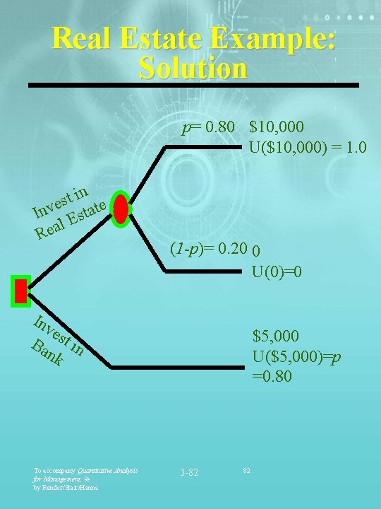
Real Estate Example: Solution p= 0. 80 $10, 000 U($10, 000) = 1. 0 in t s e Inv Estate l a e R (1 -p)= 0. 20 0 U(0)=0 Inv est Ba in nk To accompany Quantitative Analysis for Management, 9 e by Render/Stair/Hanna $5, 000 U($5, 000)=p =0. 80 3 -82 82
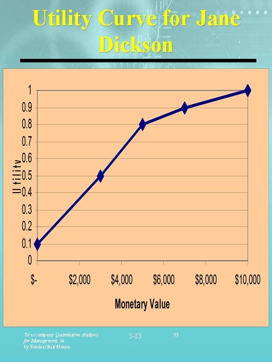
Utility Curve for Jane Dickson To accompany Quantitative Analysis for Management, 9 e by Render/Stair/Hanna 3 -83 83
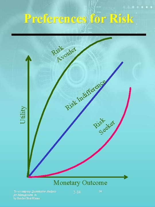
Preferences for Risk sk der i R oi Av ce n re Utility sk i R e f f i d n I sk er i R ek Se Monetary Outcome To accompany Quantitative Analysis for Management, 9 e by Render/Stair/Hanna 3 -84 84
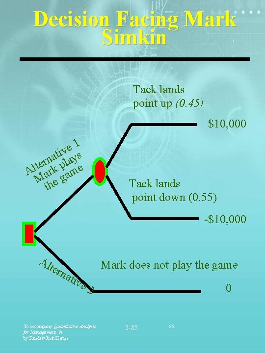
Decision Facing Mark Simkin Tack lands point up (0. 45) $10, 000 1 e v i ys t a n pla r e t Al ark ame M he g t Tack lands point down (0. 55) -$10, 000 Alt ern Mark does not play the game ativ e 2 To accompany Quantitative Analysis for Management, 9 e by Render/Stair/Hanna 0 3 -85 85
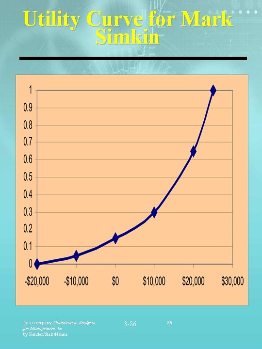
Utility Curve for Mark Simkin To accompany Quantitative Analysis for Management, 9 e by Render/Stair/Hanna 3 -86 86
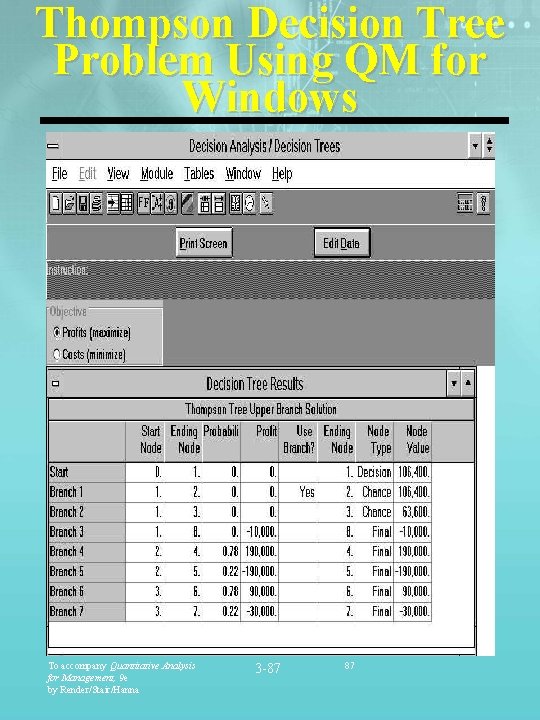
Thompson Decision Tree Problem Using QM for Windows To accompany Quantitative Analysis for Management, 9 e by Render/Stair/Hanna 3 -87 87
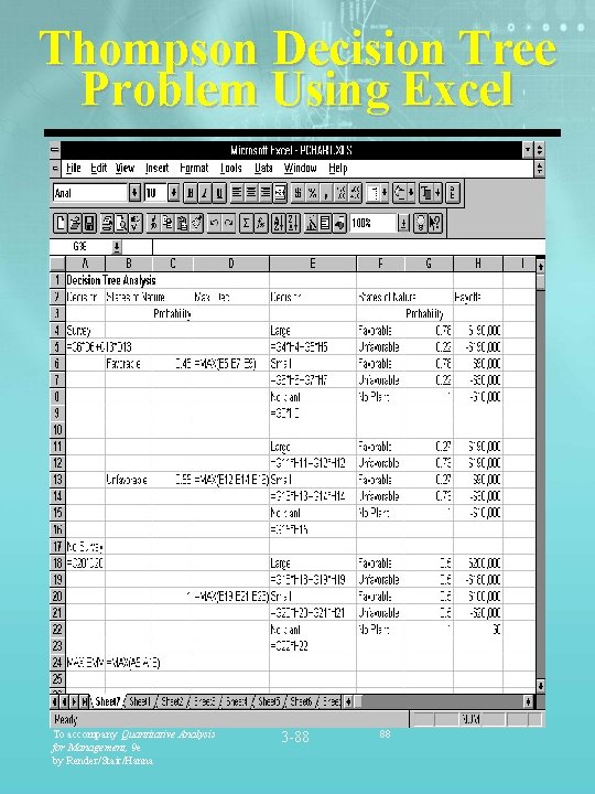
Thompson Decision Tree Problem Using Excel To accompany Quantitative Analysis for Management, 9 e by Render/Stair/Hanna 3 -88 88
- Slides: 88