Chapter 3 Database Designing What is Database Designing
Chapter : - 3 Database Designing
What is Database Designing? Each relational schema consist of a number of attributes, and the relational database schema consist of a number of relational schemas. So far we have assumed that the attributes are grouped to formed a relation schema by using a common sense of the database designer or by mapping the database schema design for a conceptual model. However we still need some formal measure of why one grouping of attributes into relation schema may be better than another.
�There are two levels at which we can discuss the goodness of relation schema. 1. Logical / Conceptual Level 2. Implementation / Storage Level v Logical Level : - q How users interprets the relation schemas and the meaning of their attributes. q Heaving a good relation schema at this level enable users to understand clearly the meaning of the data in the relations, and hence to formulate their queries correctly.
v Implementation Level : - q How the tuples in a base relation are stored and updated. q This level applies only to schemas of the base relations which will be physically stored as file whereas at logical level we are interested in schemas of both base relation or view (Virtual Relation). v As with many design problems database design may be performed using two approaches : 1. Bottom-Up Design Methodology 2. Top-Down Design Methodology
v Bottom-Up Design Methodology : Ø This methodology considers the basic relationship among individual attributes as a starting point and uses those to construct relation schema. Ø This approach is not very popular in practice because it suffer from the problem of heaving to collect a large number of binary relationships among attributes as the string point.
v Top-Down Design Methodology : Ø Also called a Design By Analysis. Ø Starts with a numbers of groupings of attributes into relations that exist together naturally, for example, on an Invoice, a form or a report. Ø The relations are then analyzed individually and collectively. Theory describe applicable to both the topdown and bottom-up design approaches, but is more practical when used with the top-down approaches.
Functional Dependency A functional dependency is a constraint between two sets of attributes from the database. Suppose our relational database schema has N attributes like A 1, A 2, A 3… AN; Let us think of whole database as being describe by a single “Universal Relational Schema” R = {A 1, A 2, A 3… AN} We don’t imply that we will actually store the database as a single table. That’s why we have to divide our database as a collection of tables. For retrieving a value of one attribute base on another attribute value we have to follow some constraints (Normalization).
Definition : - “A Functional Dependency denote by X Y between two sets of attributes X and Y that are subset of R specifies the constraints on the possible tuples that can form a relation state r of R. The constraints is that for any two tuples t 1 and t 2 in r that have t 1[X] = t 2[X] they must also have ……… t 1[Y] = t 2[Y]. ” This means that value of Y component of a tuple in r depends on or are determine by the value of X component. Alternatively the value of X component uniquely determine the value of Y component. Count…
We also say that there is a functional dependency from X to Y, or that Y is functional dependent on X. The abbreviation of Functional Dependency is FD or f. d. The set of attribute X is called the Left-hand Side of FD. The set of attribute Y is called the Right-hand Side of FD. Thus X functionally determines Y in relational schema if and only if whenever two tuples of r(R) agree on their X values, they must agree on their Y value. Count…
If a constraint on R state that there can not be more then one tuple with a given X-value in any relation instance r(R) that is X is a candidate key of R. This implies X Y for any subset of attributes Y of R. A functional dependency is a property of the semantics/meaning of attributes. The database designer will use their understanding of the semantics of the attributes of R that is how they are related to each other to specify the FD that should hold on all relation states r of R. Count…
Whenever the semantic of two sets of attributes in R indicate that a FD should hold, we specify the dependency as a constraint. The relation extension r(R) that satisfy the FD constraints are called Legal Relation State or Legal extension.
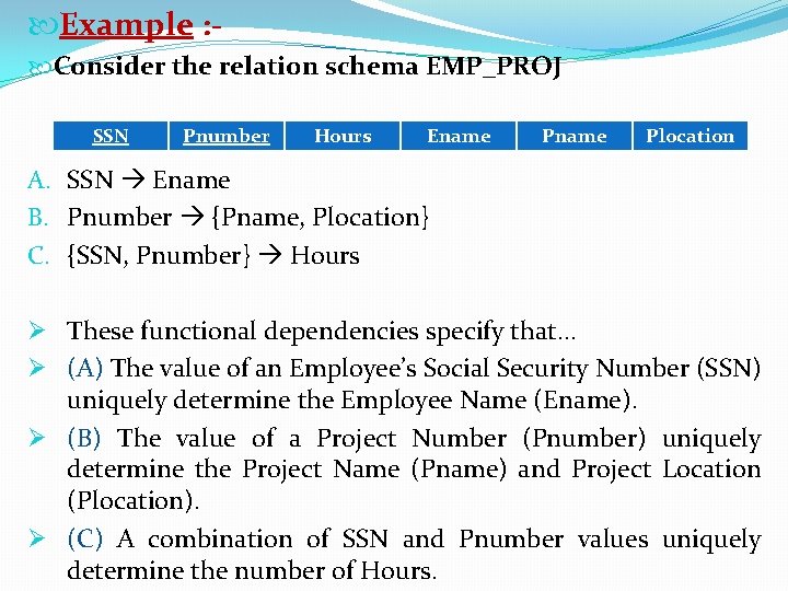
Example : Consider the relation schema EMP_PROJ SSN Pnumber Hours Ename Plocation A. SSN Ename B. Pnumber {Pname, Plocation} C. {SSN, Pnumber} Hours Ø These functional dependencies specify that… Ø (A) The value of an Employee’s Social Security Number (SSN) uniquely determine the Employee Name (Ename). Ø (B) The value of a Project Number (Pnumber) uniquely determine the Project Name (Pname) and Project Location (Plocation). Ø (C) A combination of SSN and Pnumber values uniquely determine the number of Hours.
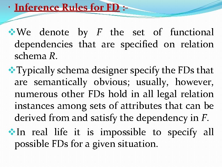
Inference Rules for FD : v. We denote by F the set of functional dependencies that are specified on relation schema R. v. Typically schema designer specify the FDs that are semantically obvious; usually, however, numerous other FDs hold in all legal relation instances among sets of attributes that can be derived from and satisfy the dependency in F. v. In real life it is impossible to specify all possible FDs for a given situation.
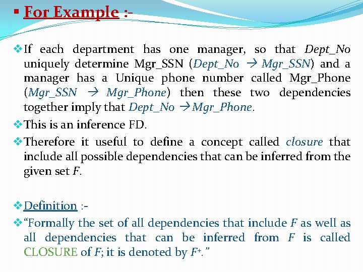
§ For Example : v If each department has one manager, so that Dept_No uniquely determine Mgr_SSN (Dept_No Mgr_SSN) and a manager has a Unique phone number called Mgr_Phone (Mgr_SSN Mgr_Phone) then these two dependencies together imply that Dept_No Mgr_Phone. v This is an inference FD. v Therefore it useful to define a concept called closure that include all possible dependencies that can be inferred from the given set F. v Definition : v “Formally the set of all dependencies that include F as well as all dependencies that can be inferred from F is called CLOSURE of F; it is denoted by F+. ”
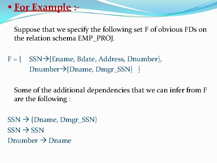
§ For Example : Suppose that we specify the following set F of obvious FDs on the relation schema EMP_PROJ. F={ SSN {Ename, Bdate, Address, Dnumber}, Dnumber {Dname, Dmgr_SSN} } Some of the additional dependencies that we can infer from F are the following : SSN {Dname, Dmgr_SSN} SSN Dnumber Dname
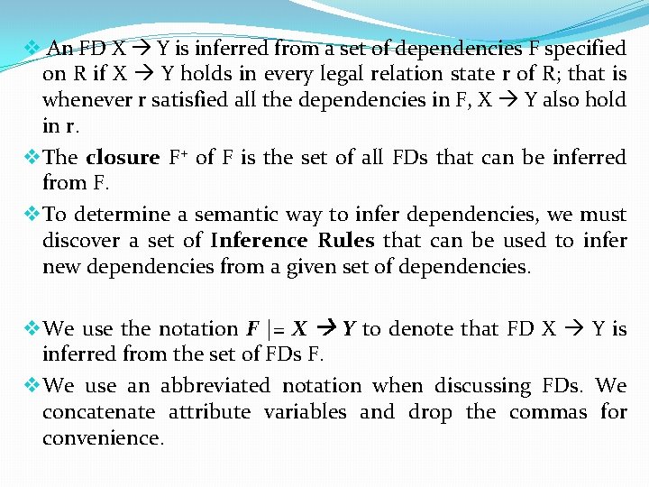
v An FD X Y is inferred from a set of dependencies F specified on R if X Y holds in every legal relation state r of R; that is whenever r satisfied all the dependencies in F, X Y also hold in r. v The closure F+ of F is the set of all FDs that can be inferred from F. v To determine a semantic way to infer dependencies, we must discover a set of Inference Rules that can be used to infer new dependencies from a given set of dependencies. v We use the notation F |= X Y to denote that FD X Y is inferred from the set of FDs F. v We use an abbreviated notation when discussing FDs. We concatenate attribute variables and drop the commas for convenience.
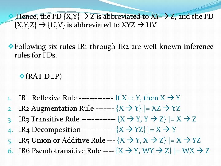
v Hence, the FD {X, Y} Z is abbreviated to XY Z, and the FD {X, Y, Z} {U, V} is abbreviated to XYZ UV v Following six rules IR 1 through IR 2 are well-known inference rules for FDs. v (RAT DUP) 1. 2. 3. 4. 5. 6. IR 1 Reflexive Rule ------- If X Y, then X Y IR 2 Augmentation Rule ------- {X Y} |= XZ YZ IR 3 Transitive Rule ------- {X Y, Y Z} |= X Z IR 4 Decomposition ------ {X YZ} |= X Y IR 5 Union or Additive Rule --- {X Y, X Z} |= X YZ IR 6 Pseudotransitive Rule ---- {X Y, WY Z} |= WX Z
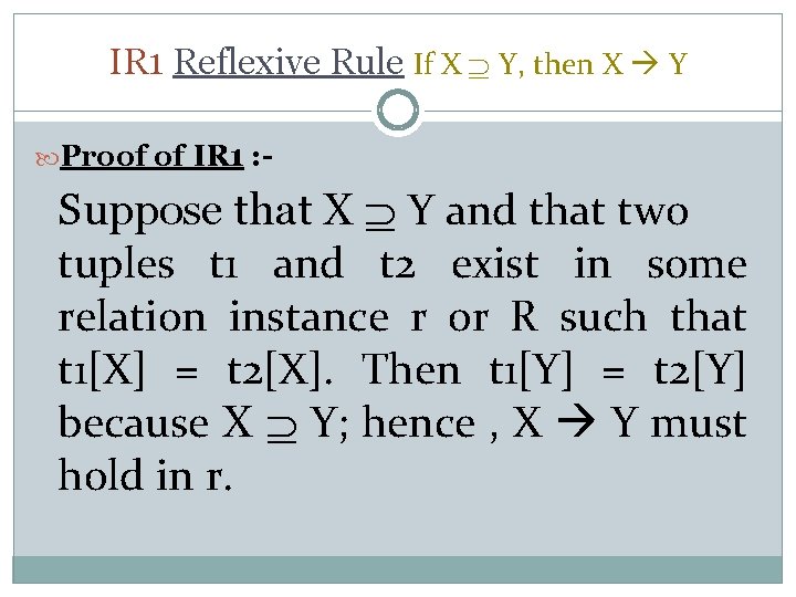
IR 1 Reflexive Rule If X Y, then X Y Proof of IR 1 : - Suppose that X Y and that two tuples t 1 and t 2 exist in some relation instance r or R such that t 1[X] = t 2[X]. Then t 1[Y] = t 2[Y] because X Y; hence , X Y must hold in r.
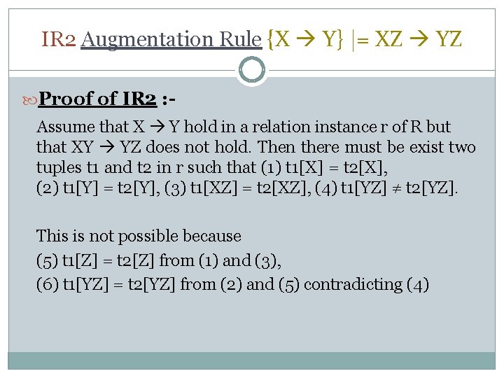
IR 2 Augmentation Rule {X Y} |= XZ YZ Proof of IR 2 : - Assume that X Y hold in a relation instance r of R but that XY YZ does not hold. Then there must be exist two tuples t 1 and t 2 in r such that (1) t 1[X] = t 2[X], (2) t 1[Y] = t 2[Y], (3) t 1[XZ] = t 2[XZ], (4) t 1[YZ] ≠ t 2[YZ]. This is not possible because (5) t 1[Z] = t 2[Z] from (1) and (3), (6) t 1[YZ] = t 2[YZ] from (2) and (5) contradicting (4)
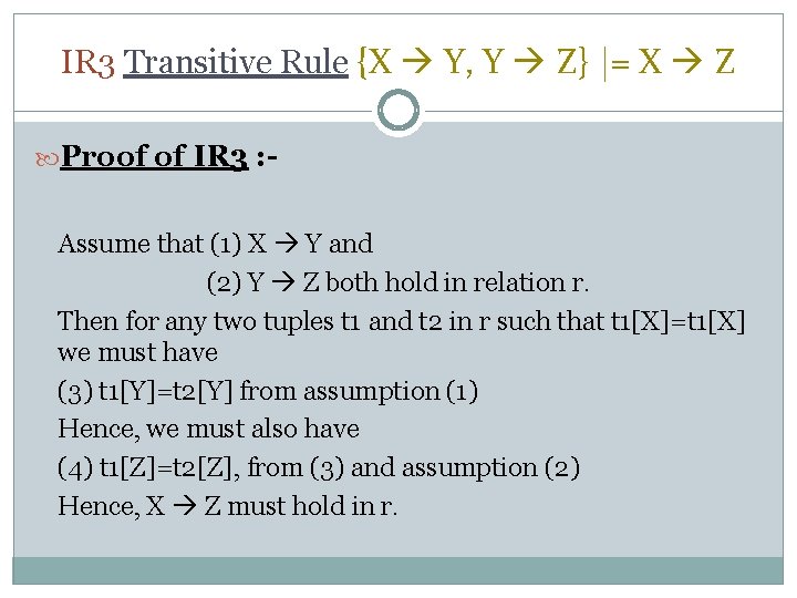
IR 3 Transitive Rule {X Y, Y Z} |= X Z Proof of IR 3 : - Assume that (1) X Y and (2) Y Z both hold in relation r. Then for any two tuples t 1 and t 2 in r such that t 1[X]=t 1[X] we must have (3) t 1[Y]=t 2[Y] from assumption (1) Hence, we must also have (4) t 1[Z]=t 2[Z], from (3) and assumption (2) Hence, X Z must hold in r.
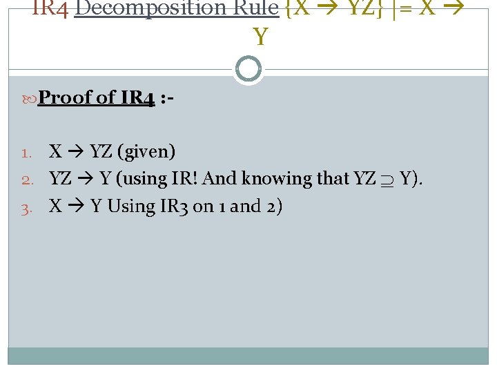
IR 4 Decomposition Rule {X YZ} |= X Y Proof of IR 4 : - X YZ (given) 2. YZ Y (using IR! And knowing that YZ Y). 3. X Y Using IR 3 on 1 and 2) 1.
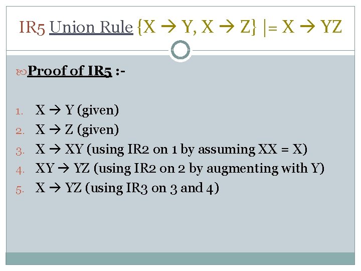
IR 5 Union Rule {X Y, X Z} |= X YZ Proof of IR 5 : 1. 2. 3. 4. 5. X Y (given) X Z (given) X XY (using IR 2 on 1 by assuming XX = X) XY YZ (using IR 2 on 2 by augmenting with Y) X YZ (using IR 3 on 3 and 4)
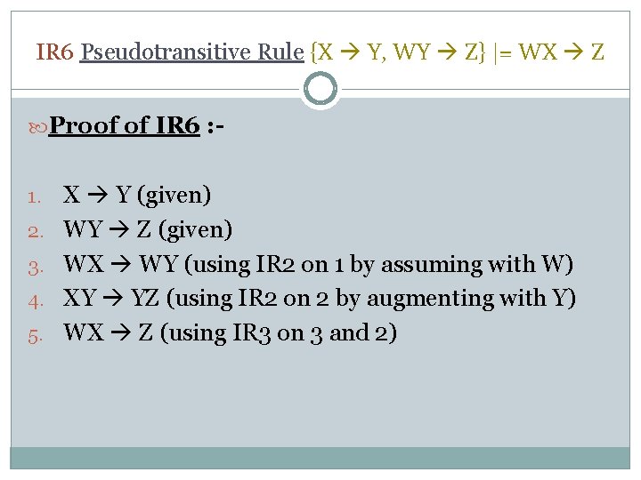
IR 6 Pseudotransitive Rule {X Y, WY Z} |= WX Z Proof of IR 6 : 1. 2. 3. 4. 5. X Y (given) WY Z (given) WX WY (using IR 2 on 1 by assuming with W) XY YZ (using IR 2 on 2 by augmenting with Y) WX Z (using IR 3 on 3 and 2)
Armstrong’s Inference Rules It has been shown by Armstrong (1947) that inference rules IR 1 Through IR 3 are sound and complete. By Sound, we mean that given a set of FDs F specified on a relation schema R , any dependency that we can infer from F by using IR 1 through IR 3 holds in every relation state r of R that satisfied the dependency in F. By Complete, we mean that using IR 1 through IR 3 repeatedly to infer dependencies until no more dependency can be inferred result in the complete set of all possible dependencies that can be inferred from F. Hence Infer Rules IR 1 through IR 3 are known as Armstrong’s Rule.
Normalization of Relation Initially Dr. E. F. Codd proposed three normal forms, which he called First Normal Form (1 NF), Second Normal Form (2 NF), Third Normal Form (3 NF). A stronger definition of 3 NF is called Boyce. Codd Normal Form(BCNF). These normal forms are based on a single analytical tool: the Functional Dependency among the attributes of relation. Later the 4 NF and 5 NF were proposed based on concept of multivalued dependency and join dependency respectively.
Normalization of Data It can be consider the process of analyzing the relation schemas based on their FDs and primary key to achieve the desirable properties of : Minimizing Redundancy and Minimizing the Insertion, Deletion and Update Unsatisfied relation schemas that do not meet certain conditions – the Normal Form Tests – are decomposed into smaller relation schemas that meet the test and hence posses the desirable properties.
Thus, the normalization producer provides database designers with the following: The formal framework for analyzing relation schemas base on their keys and on the functional dependencies among their attributes. A series of normal forms tests that can be carried out on individual relation schemas so that the relational database can be normalized to any desired degree. Definition : The NF of the relation refers highest NF condition that is meets, and hence indicate the degree to which it has been normalized.
Normal Forms when consider in isolation from, other factors, do not guarantee a good database design. It is generally not sufficient to check separately that each relation schema in the database is, say in BCNF or in 3 NF. Rather, the purpose of normalization through decomposition must also confirm the existence of additional properties that the relational schemas, taken together, should process.
This would include two properties : 1. Lossless Join or Nonadditive Join Which guarantees that the spurious tuple generation problem. 2. Dependency Preservation Which ensure that each functional dependency is represented in some individual relation resulting after decomposition. § The Nonadditive join property is extremely critical and must be achieve at any cost, whereas the dependency preservation, although desirable, is sometimes sacrificed.
First Normal Form (1 NF) 1 NF is now considered to be part of formal definition of a relation in the basic relational model. It was disallow Multivalued attributes, composite attributes and their combination. It state the domain of an attributes must include only atomic value (Simple, Indivisible values) and that the value of any attribute in a tuple must be a singled value from the domain of that attribute. The only attribute values permitted by 1 NF are single atomic or indivisible value
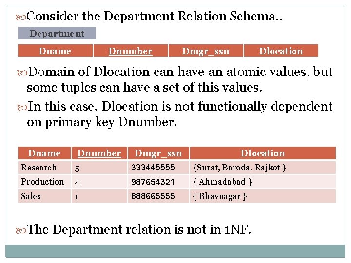
Consider the Department Relation Schema. . Department Dname Dnumber Dmgr_ssn Dlocation Domain of Dlocation can have an atomic values, but some tuples can have a set of this values. In this case, Dlocation is not functionally dependent on primary key Dnumber. Dname Dnumber Dmgr_ssn Dlocation Research 5 333445555 {Surat, Baroda, Rajkot } Production 4 987654321 { Ahmadabad } Sales 1 888665555 { Bhavnagar } The Department relation is not in 1 NF.
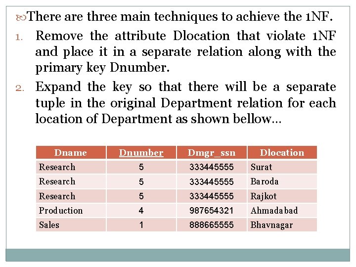
There are three main techniques to achieve the 1 NF. Remove the attribute Dlocation that violate 1 NF and place it in a separate relation along with the primary key Dnumber. 2. Expand the key so that there will be a separate tuple in the original Department relation for each location of Department as shown bellow… 1. Dname Dnumber Dmgr_ssn Dlocation Research 5 333445555 Surat Research 5 333445555 Baroda Research 5 333445555 Rajkot Production 4 987654321 Ahmadabad Sales 1 888665555 Bhavnagar
3. If a maximum number of values is known for the • • • attribute-for example, if it is known that at most three locations can exist for a department-replace the Dlocation attribute by three atomic attributes: Dlocation 1, Dlocation 2, Dlocation 3. This solution has a disadvantages of introducing NULL values if most departments have few then three locations. Of the three solution the first is generally considered best because it does not suffer from redundancy. 1 NF also disallow multivalued attributes that are themselves composite. These are called Nested Relation.
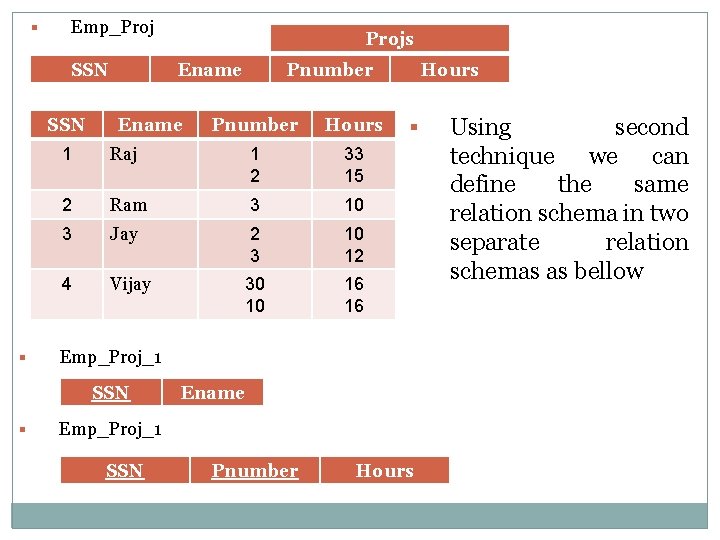
§ Emp_Proj SSN § Ename Pnumber Hours 1 Raj 1 2 33 15 2 Ram 3 10 3 Jay 2 3 10 12 4 Vijay 30 10 16 16 Hours § Emp_Proj_1 SSN § Projs Ename Emp_Proj_1 SSN Pnumber Hours Using second technique we can define the same relation schema in two separate relation schemas as bellow
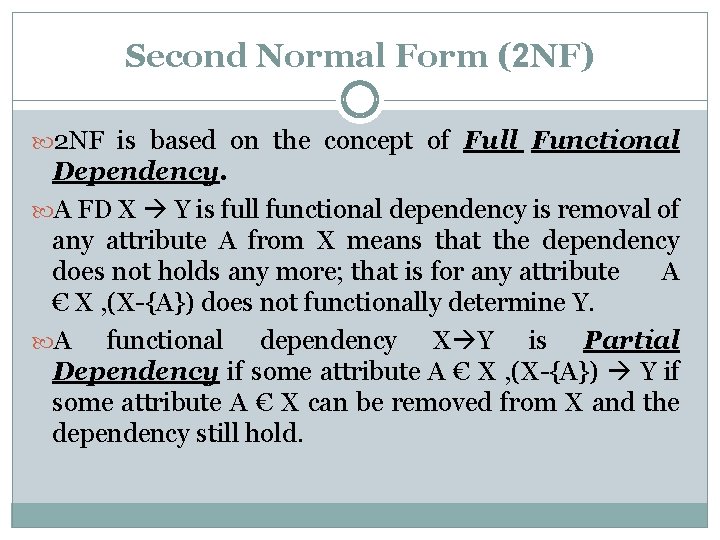
Second Normal Form (2 NF) 2 NF is based on the concept of Full Functional Dependency. A FD X Y is full functional dependency is removal of any attribute A from X means that the dependency does not holds any more; that is for any attribute A € X , (X-{A}) does not functionally determine Y. A functional dependency X Y is Partial Dependency if some attribute A € X , (X-{A}) Y if some attribute A € X can be removed from X and the dependency still hold.
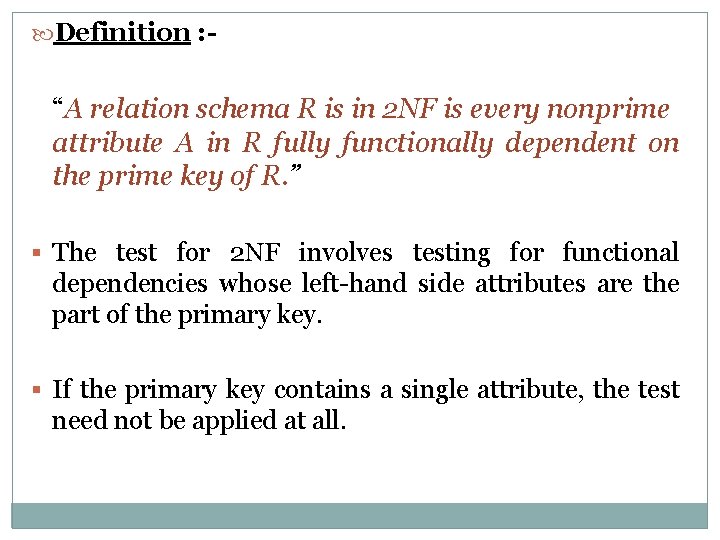
Definition : - “A relation schema R is in 2 NF is every nonprime attribute A in R fully functionally dependent on the prime key of R. ” § The test for 2 NF involves testing for functional dependencies whose left-hand side attributes are the part of the primary key. § If the primary key contains a single attribute, the test need not be applied at all.
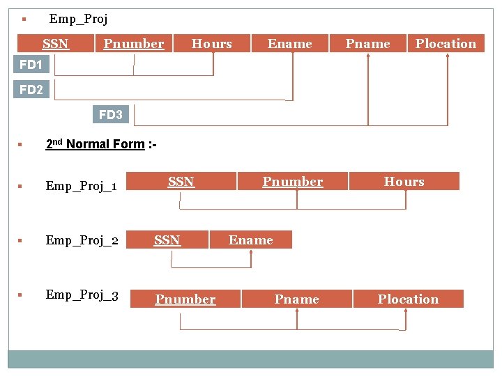
Emp_Proj § SSN Pnumber Hours Ename Plocation FD 1 FD 2 FD 3 § 2 nd Normal Form : - § Emp_Proj_1 § Emp_Proj_2 SSN § Emp_Proj_3 Pnumber SSN Pnumber Hours Ename Plocation
Third Normal Form (3 NF) 3 NF is based on the concept of Transitive Dependency. A functional Dependency X-->Y in a relation schema R is a transitive dependency if there is a set of attributes Z that is neither a candidate key nor a subset of any key of R, and both X-->Z and Z-->Y holds. The dependency SSN->Dmgr_ssn is transitive through Dnumber in EMP_DEPT. Because both the dependencies SSN->Dnumber and Dnumber->Dmgr_ssn hold and Dnumber is neither a key itself nor a subset of key of EMP_DEPT.
Definition : - “According to Codd’s original definition, a relation schema R is in 3 NF if it satisfied 2 NF and no nonprime attribute of R is the transitively dependent on the prime key. ” § The given relational schema EMP_DEPT is in 2 NF, since no partial dependencies on a key exist. § However EMP_DEPT is not in 3 NF because of the transitive dependency of Dmgr_ssn on SSN via Dnumber. § We can normalize EMP_DEPT by decomposing it in to two 3 NF relations ED 1 And ED 2 represent the independent entity facts about Employee and Department. § A JOIN operation on ED 1 and ED 2 will recover the original relation EMP_DEPT.
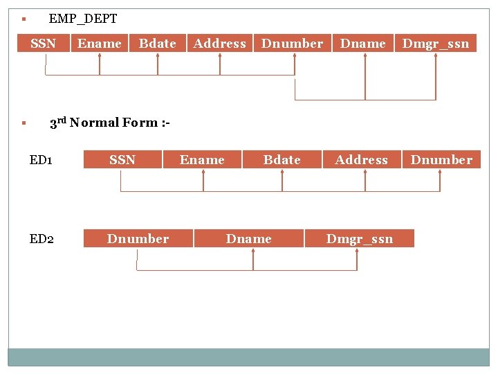
§ EMP_DEPT SSN § Ename Bdate Address Dnumber Dname Dmgr_ssn Address Dnumber 3 rd Normal Form : ED 1 SSN ED 2 Dnumber Ename Bdate Dname Dmgr_ssn
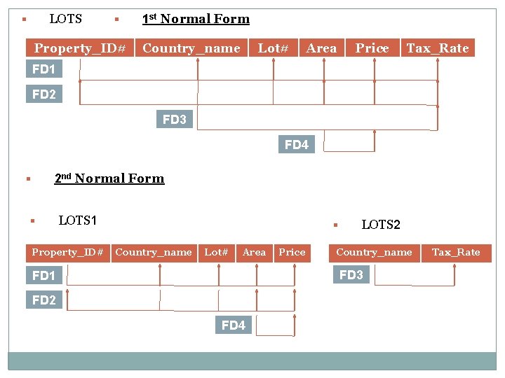
LOTS § § Property_ID# 1 st Normal Form Country_name Lot# Area Price Tax_Rate FD 1 FD 2 FD 3 FD 4 2 nd Normal Form § § LOTS 1 Property_ID# § Country_name Lot# Area Price LOTS 2 Country_name FD 3 FD 1 FD 2 FD 4 Tax_Rate
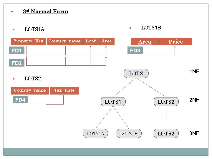
3 rd Normal Form § Property_ID# LOTS 1 B § LOTS 1 A § Country_name Lot# Area FD 1 Price FD 3 FD 2 § LOTS 2 Country_name 1 NF LOTS Tax_Rate FD 4 LOTS 1 A LOTS 1 B LOTS 2 2 NF LOTS 2 3 NF
Boyce-Codd Normal Form (BCNF) BCNF was proposed as a simpler form of 3 NF, but it was found to be stricter than 3 NF. That is every relation in BCNF is also in 3 NF; However, a relation in 3 NF is not necessary in BCNF. We can see the need for stronger NF than 3 NF in example of LOTS relation schema with its four FDs FD 1 to FD 4. Suppose we have a thousands of lots for only two countries India and USA. Suppose also that the lots size in India are of 1. 0, 1. 2 up to 2. 0.
Where as the lots size in USA are of 2. 1, 2. 2 up to 3. 0. In such a situation we have an additional functional dependency FD 5 : Area --> Country. The Area of LOTS can determine the Country. This relation can generate the redundancy by repeating the same value “India” in Country for Area = 1. 0, 1. 1, 1. 2 up to the 2. 0. For these ten values the value for Country name would be same as “India”. And same situation in Country USA. So that there is again need for decomposition of the relation schema LOTS 1 A in to two different schemas LOTS 1 AX and LOTS 1 AY.
Definition : - A relation schema R is in BCNF if whenever a nontrivial functional dependency X --> A (3 NF) holds in R, then X is super key of R. Means if we want to check that the schema is in BCNF or not for that the schema must be in 3 NF. Then after if any FD in that schema is holds that any nonprime attribute can determine the value of any prime attribute then that will violate the second pre condition for BCNF. So that to convert that schema in to BCNF again we have to decomposed that relation schema. Like. . :
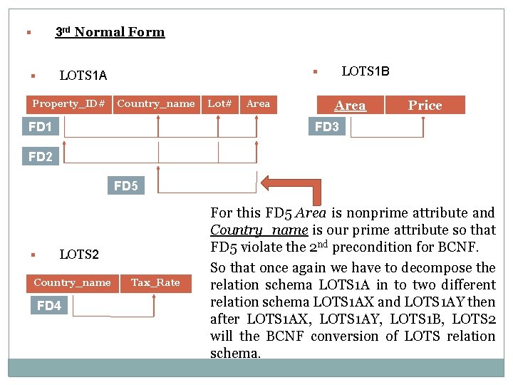
3 rd Normal Form § Property_ID# LOTS 1 B § LOTS 1 A § Country_name FD 1 Lot# Area Price FD 3 FD 2 FD 5 § LOTS 2 Country_name FD 4 Tax_Rate For this FD 5 Area is nonprime attribute and Country_name is our prime attribute so that FD 5 violate the 2 nd precondition for BCNF. So that once again we have to decompose the relation schema LOTS 1 A in to two different relation schema LOTS 1 AX and LOTS 1 AY then after LOTS 1 AX, LOTS 1 AY, LOTS 1 B, LOTS 2 will the BCNF conversion of LOTS relation schema.
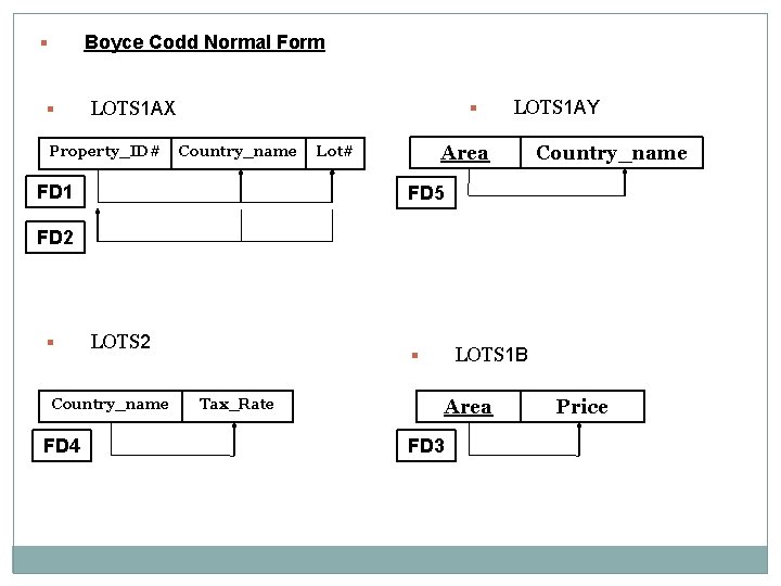
Boyce Codd Normal Form § § LOTS 1 AX Property_ID# § Country_name FD 1 LOTS 1 AY Area Lot# Country_name FD 5 FD 2 § LOTS 2 Country_name FD 4 § Tax_Rate LOTS 1 B Area FD 3 Price
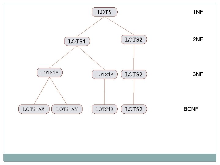
1 NF LOTS 2 2 NF LOTS 1 B LOTS 2 3 NF LOTS 1 B LOTS 2 LOTS 1 AX LOTS 1 AY BCNF
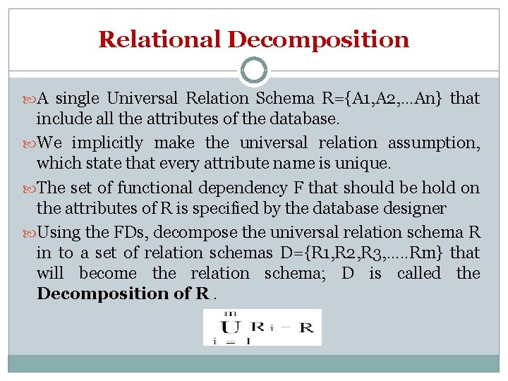
Relational Decomposition A single Universal Relation Schema R={A 1, A 2, …An} that include all the attributes of the database. We implicitly make the universal relation assumption, which state that every attribute name is unique. The set of functional dependency F that should be hold on the attributes of R is specified by the database designer Using the FDs, decompose the universal relation schema R in to a set of relation schemas D={R 1, R 2, R 3, …. . Rm} that will become the relation schema; D is called the Decomposition of R.
Properties of Relational Decomposition 1. Dependency Preservation Property : It would be useful if each FD X-->Y specified in F either appeared directly in one of the relation schema Ri in D or could be inferred from the FDs that appear in some Ri. Informally this is the Dependency Preservation Condition. It is not necessary that the exact dependency specified in F appear themselves in individual relations of the decomposition D. It is sufficient that the union of the FDs that hold on the individual relations in D be equivalent to F (set of FDs which are hold in Universal Schema R).
v Definition : - Given a set of dependencies F on R, the Projection of F in Ri where Ri is a subset of R, is the set of FDs X --> Y in F+ such that attributes in X u Y are all contain in Ri. Hence the projection of F on each relation schema Ri in the decomposition D is the set of FDs F+ the closure of F, such that all their Left-hand side and Right-hand side attributes are in Ri.
• We say that a decomposition D={R 1, R 2, R 3…, Rm} of R is Dependency. Preserving with respect to F if the union of projection of F on each Ri in D is equivalent to F+. • If a decomposition is not dependencypreserving, some dependency is Lost in the decomposition. • To check a Lost dependency holds, we must take the JOIN of to or more relations.
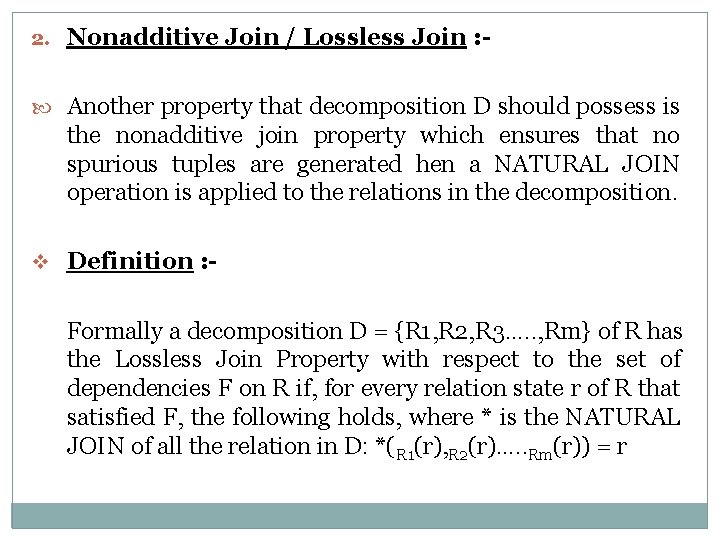
2. Nonadditive Join / Lossless Join : Another property that decomposition D should possess is the nonadditive join property which ensures that no spurious tuples are generated hen a NATURAL JOIN operation is applied to the relations in the decomposition. v Definition : - Formally a decomposition D = {R 1, R 2, R 3…. . , Rm} of R has the Lossless Join Property with respect to the set of dependencies F on R if, for every relation state r of R that satisfied F, the following holds, where * is the NATURAL JOIN of all the relation in D: *(R 1(r), R 2(r)…. . Rm(r)) = r
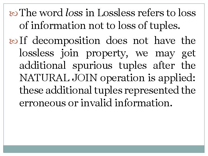
The word loss in Lossless refers to loss of information not to loss of tuples. If decomposition does not have the lossless join property, we may get additional spurious tuples after the NATURAL JOIN operation is applied: these additional tuples represented the erroneous or invalid information.
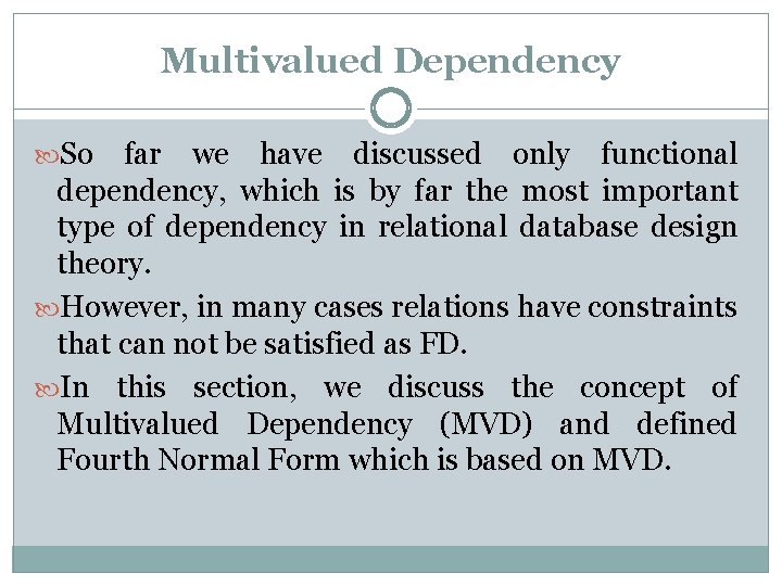
Multivalued Dependency So far we have discussed only functional dependency, which is by far the most important type of dependency in relational database design theory. However, in many cases relations have constraints that can not be satisfied as FD. In this section, we discuss the concept of Multivalued Dependency (MVD) and defined Fourth Normal Form which is based on MVD.
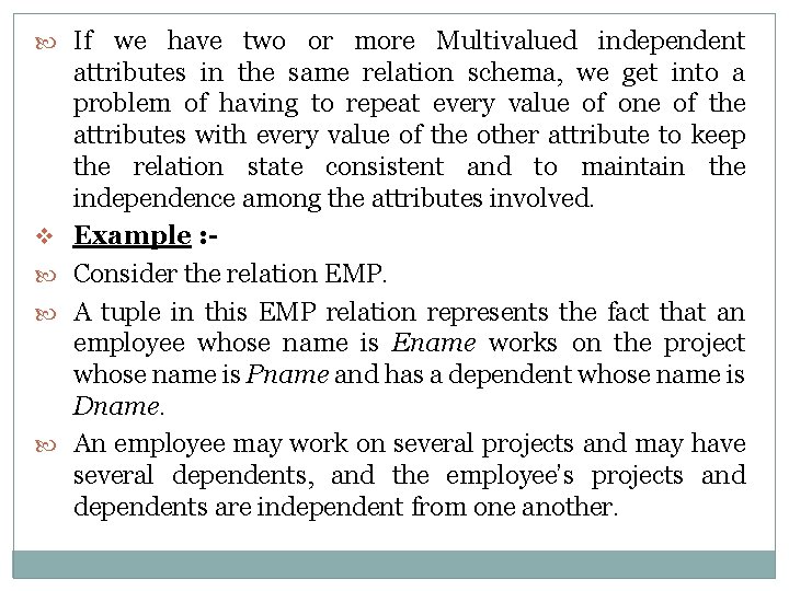
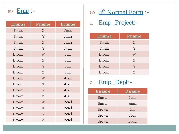
If we have two or more Multivalued independent v attributes in the same relation schema, we get into a problem of having to repeat every value of one of the attributes with every value of the other attribute to keep the relation state consistent and to maintain the independence among the attributes involved. Example : Consider the relation EMP. A tuple in this EMP relation represents the fact that an employee whose name is Ename works on the project whose name is Pname and has a dependent whose name is Dname. An employee may work on several projects and may have several dependents, and the employee’s projects and dependents are independent from one another.
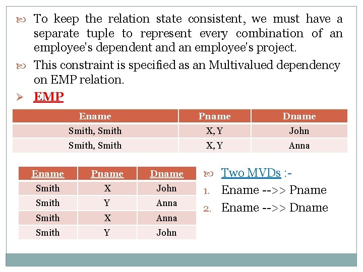
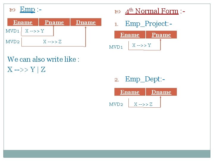
To keep the relation state consistent, we must have a separate tuple to represent every combination of an employee’s dependent and an employee’s project. This constraint is specified as an Multivalued dependency on EMP relation. Ø EMP Ename Pname Dname Smith, Smith X, Y John Smith, Smith X, Y Anna Ename Pname Dname Smith X John Smith Y Anna Smith X Anna Smith Y John Two MVDs : - Ename -->> Pname 2. Ename -->> Dname 1.
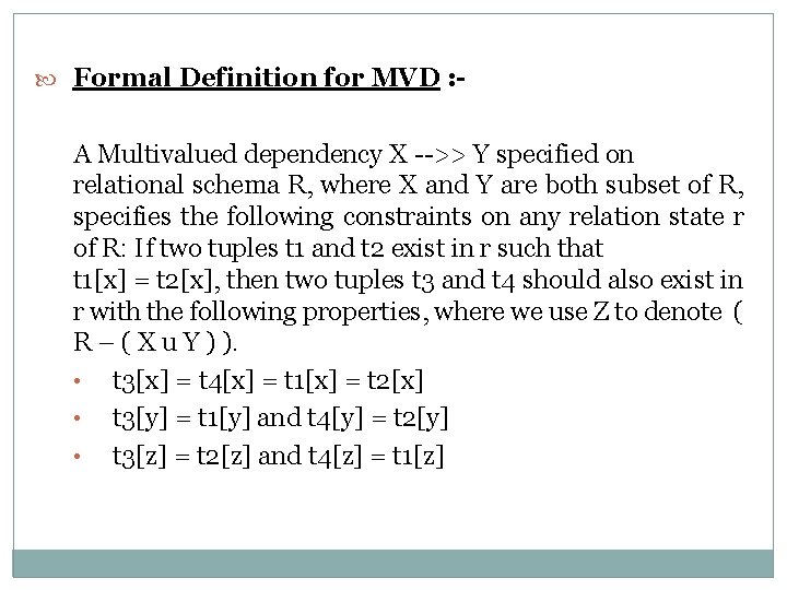
Formal Definition for MVD : - A Multivalued dependency X -->> Y specified on relational schema R, where X and Y are both subset of R, specifies the following constraints on any relation state r of R: If two tuples t 1 and t 2 exist in r such that t 1[x] = t 2[x], then two tuples t 3 and t 4 should also exist in r with the following properties, where we use Z to denote ( R – ( X u Y ) ). • t 3[x] = t 4[x] = t 1[x] = t 2[x] • t 3[y] = t 1[y] and t 4[y] = t 2[y] • t 3[z] = t 2[z] and t 4[z] = t 1[z]
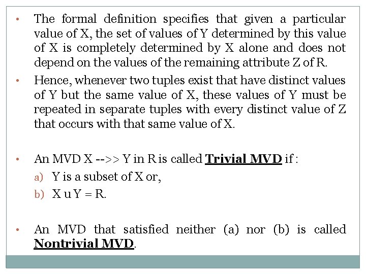
• • The formal definition specifies that given a particular value of X, the set of values of Y determined by this value of X is completely determined by X alone and does not depend on the values of the remaining attribute Z of R. Hence, whenever two tuples exist that have distinct values of Y but the same value of X, these values of Y must be repeated in separate tuples with every distinct value of Z that occurs with that same value of X. • An MVD X -->> Y in R is called Trivial MVD if : a) Y is a subset of X or, b) X u Y = R. • An MVD that satisfied neither (a) nor (b) is called Nontrivial MVD.
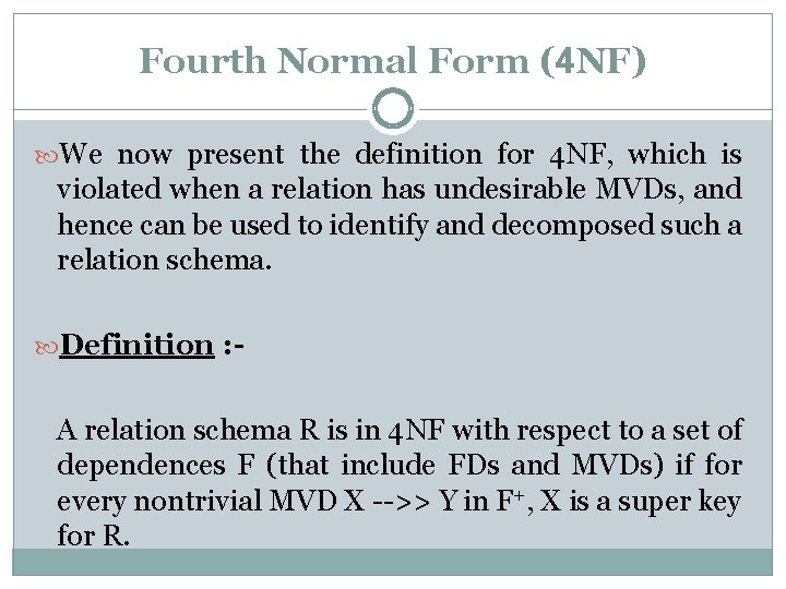
Fourth Normal Form (4 NF) We now present the definition for 4 NF, which is violated when a relation has undesirable MVDs, and hence can be used to identify and decomposed such a relation schema. Definition : - A relation schema R is in 4 NF with respect to a set of dependences F (that include FDs and MVDs) if for every nontrivial MVD X -->> Y in F+, X is a super key for R.
Emp : - 4 th Normal Form : 1. Emp_Project: - Ename Pname Dname Smith X John Smith Y Anna Ename Pname Smith X Anna Smith X Smith Y John Smith Y Brown W Jim Brown W Brown X Jim Brown X Brown Y Jim Brown Y Brown Z Jim Brown Z Brown W Joan Brown X Joan Brown Y Joan Ename Dname Brown Z Joan Smith John Brown W Bond Smith Anna Brown X Bond Brown Jim Brown Y Bond Brown Joan Brown Z Bond Brown Bond 2. Emp_Dept: -
Emp : - 4 th Normal Form : - Ename MVD 1 MVD 2 Pname Dname X -->> Y X -->> Z Emp_Project: - 1. Ename MVD 1 Pname X -->> Y We can also write like : X -->> Y | Z 2. Emp_Dept: Ename MVD 2 Dname X -->> Z
Join Dependency and Fifth Normal Form There may be no FD in R that violate any NF up to BCNF, and there may be no nontrivial MVD present in R that violate 4 NF. We then resort to another dependency called Join Dependency and, if it is present, carry out a multiway decomposition into 5 NF. Such a dependency is very difficult to detect in practice; therefore normalization in 5 th Normal Form is very rarely done in practice.
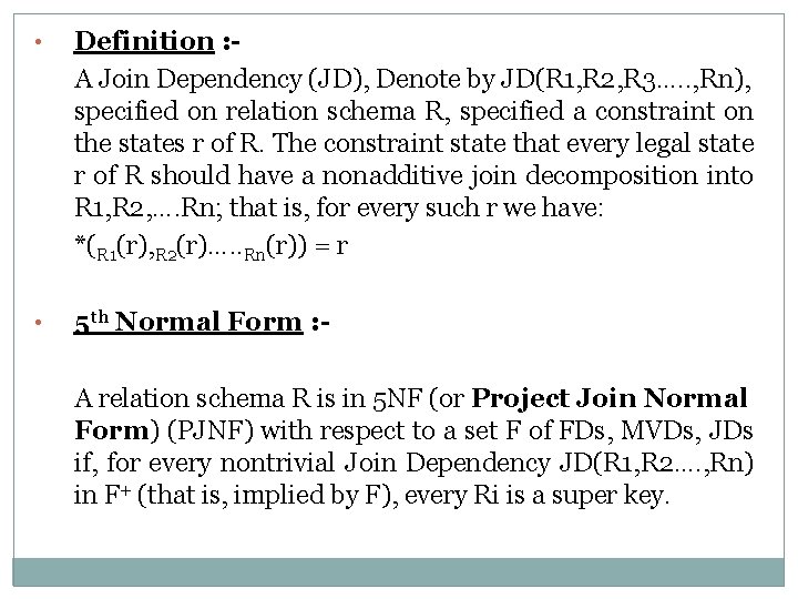
• Definition : A Join Dependency (JD), Denote by JD(R 1, R 2, R 3…. . , Rn), specified on relation schema R, specified a constraint on the states r of R. The constraint state that every legal state r of R should have a nonadditive join decomposition into R 1, R 2, …. Rn; that is, for every such r we have: *(R 1(r), R 2(r)…. . Rn(r)) = r • 5 th Normal Form : A relation schema R is in 5 NF (or Project Join Normal Form) (PJNF) with respect to a set F of FDs, MVDs, JDs if, for every nontrivial Join Dependency JD(R 1, R 2…. , Rn) in F+ (that is, implied by F), every Ri is a super key.
Design Phases For small Application it may be feasible fro a database designer who understand the application requirements to decide directly on the relations to be created, their attributes and the constraints on the relations. However such a direct design process is difficult for real-world applications. Often no one can understand the complete data need of an application. The database designer must interact with the users of the application to understand the needs of the application, represent them in a high-level fashion that can be understand by the users.
And finally translate the requirement into a lower levels of the design. The data is the requirement of the users and database structure fulfills these requirements. Following are the sequential tasks to be performed while designing database : 1. Collect Database Requirements. 2. Decide the Number of Entities and their Attributes. 3. Make Relationships between Entities. 4. Conceptual Designing. 5. Logical Designing. 6. Physical Designing.
q. The main phases of database designing : 1. Requirements and Data : - The initial phase of the database designing is to characterized fully the data needs of the database users. The database designer needs to interact extensively with domain experts and users to carry out this task. The outcome of this phase is specification of user requirements.
2. Choose Data Model : - Next, the designer chooses the data model and by applying the concept of the data model, translate these requirements into a conceptual schema of the database. Schema developed at this conceptualdesign phase provides a detail overview of the enterprise. The entity relationship model is typically used to represent the conceptual design. Typically, the conceptual-design phase result in the creation of the E-R diagram that provide the graphic representation of the schema.
3. Functional Requirements : - A fully developed conceptual schema also indicates the functional requirements of the enterprise. In a specification of Functional Requirements user describe the kinds of operations (Transactions) that will be performed on the data like : • Modifying and Updating Data. • Searching and Retrieving Data. • Deleting Data.
Process of moving from an abstract data model to the implementation of the database processes in two final design phases : • Logical-design phase • Physical-design phase 1. Logical-design Phase : The designer maps the high-level conceptual schema into the implementation data model of the database system that will be used. The implementation data model is typically the relational data model, and this step consists of mapping the conceptual schema defined using the entity-relationship model into a relational schem.
2. Physical-design Phase : - Finally the database designer use the resulting system specific database schema in the subsequent physicaldesign phase, in which the physical features of the database are specified. These features include the form of file organization and the internal storage structure. • The physical schema of a database can be change easily after an application has been built. However changes to the logical schema are usually harder to carry out, since they may affect the number of queries and update scattered across application code.
- Slides: 71