Chapter 3 Data Exploration and Dimension Reduction Data

Chapter 3 – Data Exploration and Dimension Reduction Data Mining for Business Intelligence Shmueli, Patel & Bruce © Galit Shmueli and Peter Bruce 2008

Exploring the data Statistical summary of data: common metrics Average Median Minimum Maximum Standard deviation Counts & percentages

Summary Statistics – Boston Housing

Correlation Analysis Below: Correlation matrix for portion of Boston Housing data Shows correlation between variable pairs

Matrix Plot 1 9 Shows scatterplots for variable pairs 0. 2 0. 4 0. 6 0. 8 1. 8 3. 6 5. 4 7. 2 0 ZN 102 0. 6 1. 2 1. 8 2. 4 3 0 INDUS 101 0 Example: scatterplots for 3 Boston Housing variables 0. 2 0. 4 0. 6 0. 8 1 0 CRIM 101 0 1. 8 3. 6 5. 4 7. 2 9 0 0. 6 1. 2 1. 8 2. 4 3

Principal Components Analysis Goal: Reduce a set of numerical variables. The idea: Remove the overlap of information between these variable. [“Information” is measured by the sum of the variances of the variables. ] Final product: a smaller number of numerical variables that contain most of the information

Principal Components Analysis How does PCA do this? Create new variables that are linear combinations of the original variables (i. e. , they are weighted averages of the original variables). These linear combinations are uncorrelated (no information overlap), and only a few of them contain most of the original information. The new variables are called principal components.

Example – Breakfast Cereals

Consider calories & ratings Total variance (=“information”) is sum of individual variances: 379. 63 + 197. 32 Calories accounts for 379. 63/197. 32 = 66%

First & Second Principal Components Z 1 and Z 2 are two linear combinations Z 1 has the highest variation (spread of values) Z 2 has the lowest variation

PCA output for these 2 variables Top: weights to project original data onto z 1 & z 2 e. g. (-0. 847, 0. 532) are weights for z 1 Bottom: reallocated variance for new variables z 1: 86% of total variance z 2: 14%

Principal Component Scores Weights are used to compute the above scores e. g. , col. 1 scores are computed z 1 scores using weights (-0. 847, 0. 532)

Properties of the resulting variables New distribution of information: New variances = 498 (for z 1) and 79 (for z 2) Sum of variances = sum of variances for original variables calories and ratings New variable z 1 has most of the total variance, might be used as proxy for both calories and ratings z 1 and z 2 have correlation of zero (no information overlap)

Normalizing data When a variable’s scale is greater than almost all other variables, its variance will be a dominant component of the total variance Normalize each variable to remove scale effect Divide by std. deviation (may subtract mean first) Normalization (= standardization) is usually performed in PCA; otherwise measurement units affect results When data is normalized, PC works on correlation matrix rather than covariance matrix Each variable has zero means and 1 standard deviation when it is normalized

Generalization X 1, X 2, X 3, … Xp, original p variables Z 1, Z 2, Z 3, … Zp, weighted averages of original variables i. e. Z 1 =a 1 X 1+ a 2 X 2 +a 3 X 3 +…+ ap Xp All pairs of Z variables have 0 correlation Order Z’s by variance (z 1 largest, Zp smallest) Usually the first few Z variables contain most of the information, and so the rest can be dropped.

Principal Component(PC) Analysis Data Collection Step 1 Run PC Analysis Step 2 Determine the Number of PC Step 3

Procedure for Conducting a Factor Analysis Rotate PC Step 4 Interpret PC Step 5 Calculate PC Score Step 6 Do Other Stuff Step 7

How many Factors (PC) do you Choose? Look at the Eigen Values of the PC If K of P factors have an eigen value > 1 then K PC will do a pretty good job Scree plot helpful

Scree Plot: Selection of # of Factors 6 5 4 “elbow” 3 2 1 2 4 6 8 10

Case I: Measurement of Department Store Image Description of the Research Study: To compare the images of 5 department stores in Chicago area -- Marshal Fields, Lord & Taylor, J. C. Penny, T. J. Maxx and Filene’s Basement Focus Group studies revealed several words used by respondents to describe a department store e. g. spacious/cluttered, convenient, decor, etc. Survey questionnaire used to rate the department stores using 7 point scale

Portion of Items Used to Measure Department Store Image

Measurement: Input Data Respondents … … … Store 1 Store 2 Store 3 … … … Store 4 Store 5 Attribute 1 … Attribute 10

Pair-wise Correlations among the Items Used to Measure Department Store Image X 1 X 2 X 3 X 4 X 5 X 6 X 7 X 8 X 9 X 10 1. 00 0. 79 0. 41 0. 26 0. 12 0. 89 0. 87 0. 32 0. 18 1. 00 0. 32 0. 21 0. 20 0. 90 0. 83 0. 31 0. 35 0. 23 1. 00 0. 80 0. 76 0. 34 0. 40 0. 82 0. 78 0. 72 1. 00 0. 75 0. 30 0. 28 0. 78 0. 81 0. 80 1. 00 0. 11 0. 23 0. 74 0. 77 0. 83 1. 00 0. 78 0. 30 0. 39 0. 16 1. 00 0. 29 0. 26 0. 17 1. 00 0. 82 0. 78 1. 00 0. 77 1. 00

Principal Components Analysis for the Department Store Image Data : Variance Explained by Each Factor (Latent Root) Factor 1 Factor 2 Factor 3 Factor 4 Factor 5 Factor 6 Factor 7 Factor 8 Factor 9 Factor 10 Variance Explained 5. 725 2. 761 0. 366 0. 357 0. 243 0. 212 0. 132 0. 123 0. 079 0. 001

Scree Plot: Selection of # of Factors 6 5 4 “elbow” 3 2 1 2 4 6 8 10

Unrotated Factor Loading Matrix for Department Store Image Data Using Two Factors

Unrotated Factors 1 0, 8 0, 6 0, 4 0, 2 0 -1 -0, 8 -0, 6 -0, 4 -0, 2 0 -0, 2 -0, 4 -0, 6 -0, 8 -1 0, 2 0, 4 0, 6 0, 8 1

Orthogonal Factor Rotation Unrotated Factor II +1. 0 Rotated Factor II V 1 V 2 +. 50 -1. 0 -. 50 0 Unrotated Factor I +. 50 +1. 0 V 3 V 4 -. 50 V 5 -1. 0 Rotated Factor I

Factor Loading Matrix for Department Store Image Data after Rotation of the Two Using Varimax

Rotated Factors 1 0, 8 0, 6 0, 4 0, 2 0 -1 -0, 8 -0, 6 -0, 4 -0, 2 0 -0, 2 -0, 4 -0, 6 -0, 8 -1 0, 2 0, 4 0, 6 0, 8 1

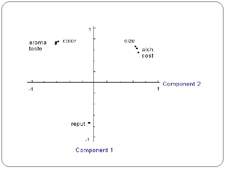
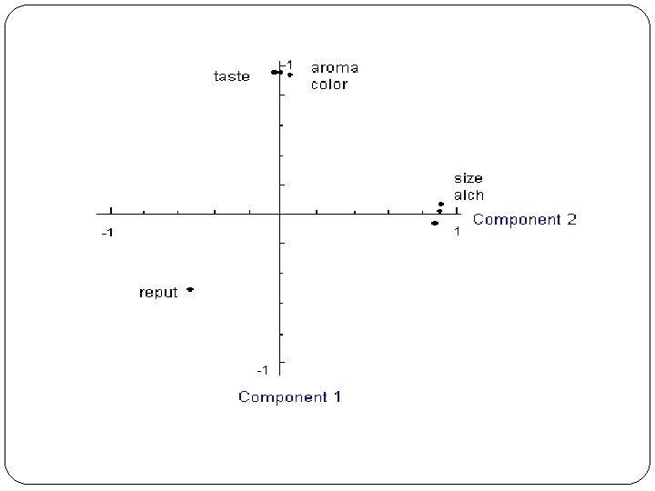
Case II: Beer Data Suppose I am interested in what influences a consumer’s choice behavior when she is shopping for beer. How important she considers each of these qualities when deciding whether or not to buy the six pack: low COST of the six pack, high SIZE of the bottle (volume), high percentage of ALCOHOL in the beer, the REPUTATION of the brand, the COLOR of the beer, nice AROMA of the beer, and good TASTE of the beer.

Correlation Matrix COST SIZE ALCOHOLREPUTAT COLOR AROMA TASTE 1 0. 54 -0. 11 -0. 26 -0. 14 0. 11 0. 54 1 0. 81 0. 11 0. 5 0. 06 -0. 44 ALCOHOL -0. 11 0. 81 1 -0. 23 -0. 38 0. 06 0. 31 REPUTAT -0. 26 0. 11 -0. 23 1 0. 23 -0. 29 -0. 26 COLOR -0. 1 0. 5 -0. 38 0. 23 1 0. 57 0. 69 AROMA -0. 14 0. 06 -0. 29 0. 57 1 0. 09 TASTE 0. 11 -0. 44 0. 31 -0. 26 0. 69 0. 09 1 SIZE

Variance Explained by Each Factor Axis Eigen value % explained % cumulated 1 3. 31289 47. 33% 2 2. 615816 37. 37% 84. 70% 3 0. 574629 8. 21% 92. 90% 4 0. 23988 3. 43% 96. 33% 5 0. 134456 1. 92% 98. 25% 6 0. 085443 1. 22% 99. 47% 7 0. 036887 0. 53% 100. 00% Tot. 7 - -

Unrotated factor loadings 1 2 COST 0. 55 0. 73 SIZE 0. 67 0. 68 ALCOHOL 0. 63 0. 7 REPUTAT -0. 74 -0. 07 COLOR 0. 76 -0. 57 AROMA 0. 74 -0. 61 TASTE 0. 71 -0. 61 COMPONENT

Rotated Factor Loading COMPONENT 1 2 TASTE 0. 96 -0. 03 AROMA 0. 96 0. 01 COLOR 0. 95 0. 06 SIZE 0. 07 0. 95 ALCOHOL 0. 02 0. 94 COST -0. 06 0. 92 REPUTAT -0. 51 -0. 53

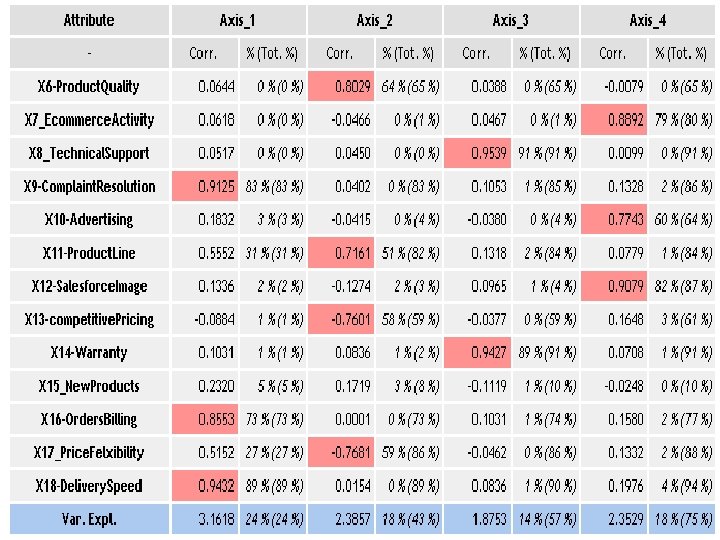
Case III: HBAT sellls paper products to magazine and service industry Survey asks perception of customer about HBAT’s performance on 13 attributes

Performance Perceptions Variables

Axis Eigen value % explained % cumulated 1 3. 83533 29. 50% 2 2. 675018 20. 58% 50. 08% 3 1. 721566 13. 24% 63. 32% 4 1. 543819 11. 88% 75. 20% 5 0. 969178 7. 46% 82. 65% 6 0. 574876 4. 42% 87. 08% 7 0. 489193 3. 76% 90. 84% 8 0. 421405 3. 24% 94. 08% 9 0. 288298 2. 22% 96. 30% 10 0. 190079 1. 46% 97. 76% 11 0. 154735 1. 19% 98. 95% 12 0. 127737 0. 98% 99. 93% 13 0. 008767 0. 07% 100. 00% Tot. 13 - -

Summary Data summarization is an important for data exploration Data summaries include numerical metrics (average, median, etc. ) and graphical summaries Data reduction is useful for compressing the information in the data into a smaller subset Principal components analysis transforms an original set of numerical data into a smaller set of weighted averages of the original data that contain most of the original information in less variables.