Chapter 3 Data Collection and Preliminary Data Analysis

Chapter 3: Data Collection and Preliminary Data Analysis 3. 1 Generalized measurement system 3. 2 Performance characteristics of sensors and sensing systems 3. 3 Data validation and preparation 3. 4 Descriptive measures of sample data 3. 5 Plotting data 3. 6 Overall measurement uncertainty 3. 7 Propagation of errors 3. 8 Planning a non-intrusive field experiment Chap 3 -Data Analysis-Reddy 1

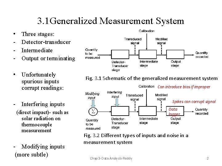
3. 1 Generalized Measurement System • - Three stages: Detector-transducer Intermediate Output or terminating • Unfortunately spurious inputs corrupt readings: Fig. 3. 1 Schematic of the generalized measurement system Can introduce bias if improper Spikes can corrupt signal - Interfering inputs (direct impact)- such as solar radiation on thermocouple measurement - Modifying inputs (more subtle) Data logger Fig. 3. 2 Different types of inputs and noise in a measurement system Chap 3 -Data Analysis-Reddy 2

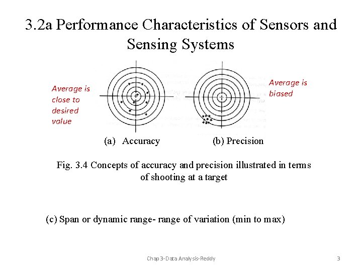
3. 2 a Performance Characteristics of Sensors and Sensing Systems Average is biased Average is close to desired value (a) Accuracy (b) Precision Fig. 3. 4 Concepts of accuracy and precision illustrated in terms of shooting at a target (c) Span or dynamic range- range of variation (min to max) Chap 3 -Data Analysis-Reddy 3

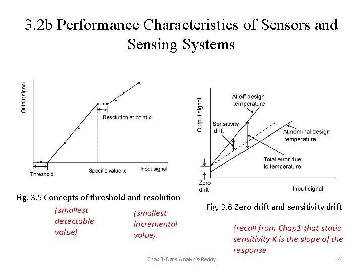
3. 2 b Performance Characteristics of Sensors and Sensing Systems Fig. 3. 5 Concepts of threshold and resolution (smallest detectable incremental value) Fig. 3. 6 Zero drift and sensitivity drift Chap 3 -Data Analysis-Reddy (recall from Chap 1 that static sensitivity K is the slope of the response 4

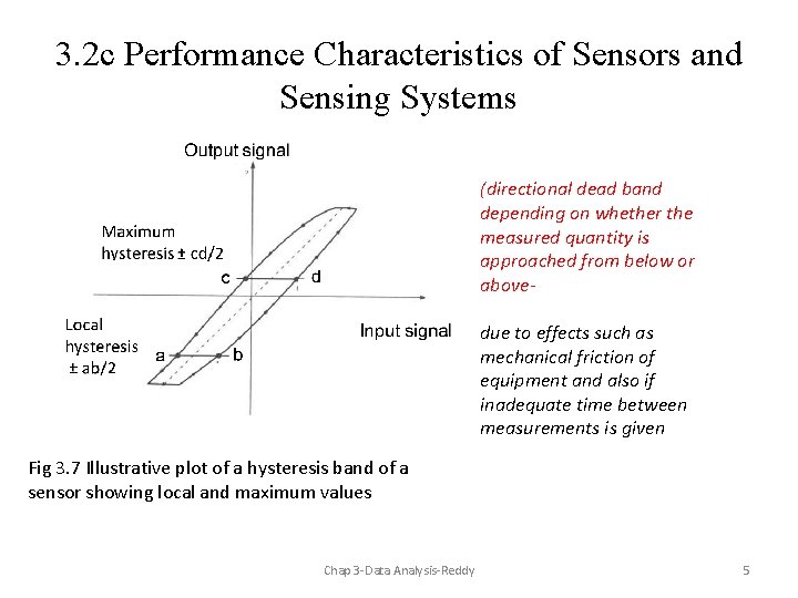
3. 2 c Performance Characteristics of Sensors and Sensing Systems (directional dead band depending on whether the measured quantity is approached from below or abovedue to effects such as mechanical friction of equipment and also if inadequate time between measurements is given Fig 3. 7 Illustrative plot of a hysteresis band of a sensor showing local and maximum values Chap 3 -Data Analysis-Reddy 5

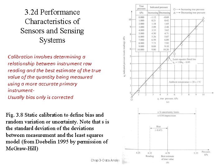
3. 2 d Performance Characteristics of Sensors and Sensing Systems Calibration involves determining a relationship between instrument raw reading and the best estimate of the true value of the quantity being measured using a more accurate primary instrument. Usually bias only is corrected Fig. 3. 8 Static calibration to define bias and random variation or uncertainty. Note that s is the standard deviation of the deviations between measurement and the least squares model (from Doebelin 1995 by permission of Mc. Graw-Hill) Chap 3 -Data Analysis-Reddy 6

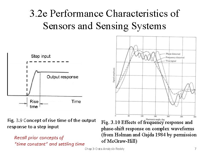
3. 2 e Performance Characteristics of Sensors and Sensing Systems Fig. 3. 9 Concept of rise time of the output response to a step input Recall prior concepts of “time constant” and settling time Fig. 3. 10 Effects of frequency response and phase-shift response on complex waveforms (from Holman and Gajda 1984 by permission of Mc. Graw-Hill) Chap 3 -Data Analysis-Reddy 7

3. 2. 2 Types and Categories of Measurements A primary measurement: one that is obtained directly from the measurement sensor. The basic criterion is that a primary measurement is of a single item from a specific measurement device. A derived measurement is one that is calculated using one or more measurements either primary or derived Further, measurements can also be categorized by type: • Stationary data does not change with time (mass of water in a tank, the area of a room, …) • Time dependent data varies with time (pollutant concentration in a water stream, temperature of a space, the chilled water flow to a building. Further, one differentiates: - Time-series data consist of a multiplicity of data taken at a single point or location over fixed intervals of time, thus retaining the time sequence nature. - Cross-sectional data are data taken at single or multiple points at a single instant in time with time not being a variable in the process. Chap 3 -Data Analysis-Reddy 8

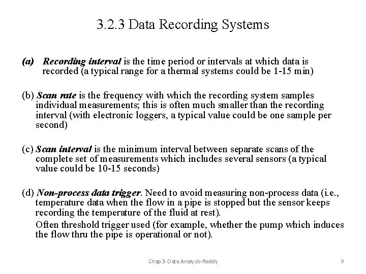
3. 2. 3 Data Recording Systems (a) Recording interval is the time period or intervals at which data is recorded (a typical range for a thermal systems could be 1 -15 min) (b) Scan rate is the frequency with which the recording system samples individual measurements; this is often much smaller than the recording interval (with electronic loggers, a typical value could be one sample per second) (c) Scan interval is the minimum interval between separate scans of the complete set of measurements which includes several sensors (a typical value could be 10 -15 seconds) (d) Non-process data trigger. Need to avoid measuring non-process data (i. e. , temperature data when the flow in a pipe is stopped but the sensor keeps recording the temperature of the fluid at rest). Often threshold trigger used (for example, whether the pump which induces the flow thru the pipe is operational or not). Chap 3 -Data Analysis-Reddy 9

3. 3 a Data Validation and Preparation Data Reduction- process of distilling raw data into a form that is suitable for subsequent analysis (a) averaging involves removing gross or egregious errors (b) limit checks: - physical limits: relative humidity <=100% - expected limits: indoor air relative humidity 30 -60% - theoretical limits: efficiency of power plant < Carnot (c) Independent/ consistency checks involving mass and energy balances (it is advisable to have redundancy) Chap 3 -Data Analysis-Reddy 10

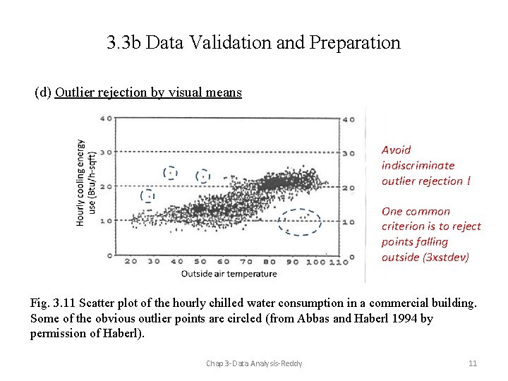
3. 3 b Data Validation and Preparation (d) Outlier rejection by visual means Avoid indiscriminate outlier rejection ! One common criterion is to reject points falling outside (3 xstdev) Fig. 3. 11 Scatter plot of the hourly chilled water consumption in a commercial building. Some of the obvious outlier points are circled (from Abbas and Haberl 1994 by permission of Haberl). Chap 3 -Data Analysis-Reddy 11

3. 3 b Data Validation and Preparation (e) Handling missing data (a) Use observations with complete data only: simplest and most obvious, and is adopted in most analysis. Many of the software programs allow such cases to be handled. Instead of coding missing values as zero, analysts often use a default value such as -99 to indicate a missing value. This approach is best suited when the missing data fraction is small enough not to cause the analysis to become biased. (b) Reject variables: In case only one or a few channels indicate high levels of missing data, the judicious approach is to drop these variables from the analysis itself. If these variables are known to be very influential, then more data needs to be collected with the measurement system modified to avoid such future occurrences. Chap 3 -Data Analysis-Reddy 12

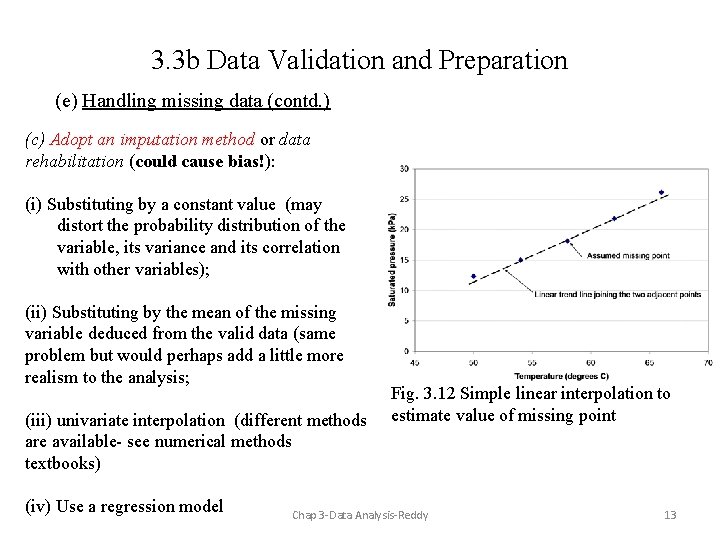
3. 3 b Data Validation and Preparation (e) Handling missing data (contd. ) (c) Adopt an imputation method or data rehabilitation (could cause bias!): (i) Substituting by a constant value (may distort the probability distribution of the variable, its variance and its correlation with other variables); (ii) Substituting by the mean of the missing variable deduced from the valid data (same problem but would perhaps add a little more realism to the analysis; (iii) univariate interpolation (different methods are available- see numerical methods textbooks) (iv) Use a regression model Fig. 3. 12 Simple linear interpolation to estimate value of missing point Chap 3 -Data Analysis-Reddy 13

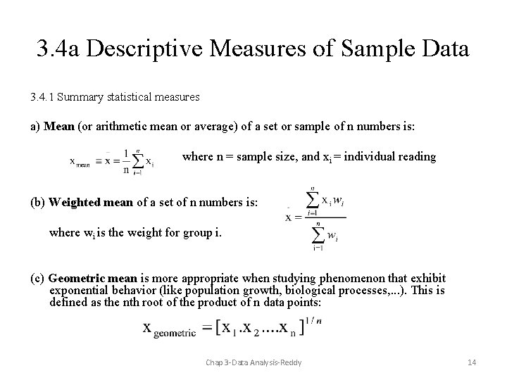
3. 4 a Descriptive Measures of Sample Data 3. 4. 1 Summary statistical measures a) Mean (or arithmetic mean or average) of a set or sample of n numbers is: where n = sample size, and xi = individual reading (b) Weighted mean of a set of n numbers is: where wi is the weight for group i. (c) Geometric mean is more appropriate when studying phenomenon that exhibit exponential behavior (like population growth, biological processes, . . . ). This is defined as the nth root of the product of n data points: Chap 3 -Data Analysis-Reddy 14

3. 4 b Descriptive Measures of Sample Data 3. 4. 1 Summary statistical measures (d) Mode is the value of the variate which occurs most frequently. When the variate is discrete, the mean may turn out to have a value that cannot actually be taken by the variate. In case of continuous variates, the mode is the value where the frequency density is highest. For example, a survey of the number of occupants in a car during the rush hour could yield a mean value of 1. 6 which is not physically possible. In such cases, using a value of 2 (i. e. , the mode) is more appropriate. (e) Median is the middle value of the variates, i. e. , half the numbers have numerical values below the median and half above. The mean is unduly influenced by extreme observations, and in such cases the median is a more robust indicator of the central tendency of the data. In case of an even number of observations, the mean of the middle two numbers is taken to be the median. (f) Range is the difference between the largest and the smallest observation values. (g) Percentiles are used to separate the data into bins. Let p be a number between 0 and 1. Then, the (100 p)th percentile (also called pth quantile), represents the data value where 100 p% of the data values are lower. Thus, 90% of the data will be below the 90 th percentile, and the median is represented by the 50 th percentile. Chap 3 -Data Analysis-Reddy 15

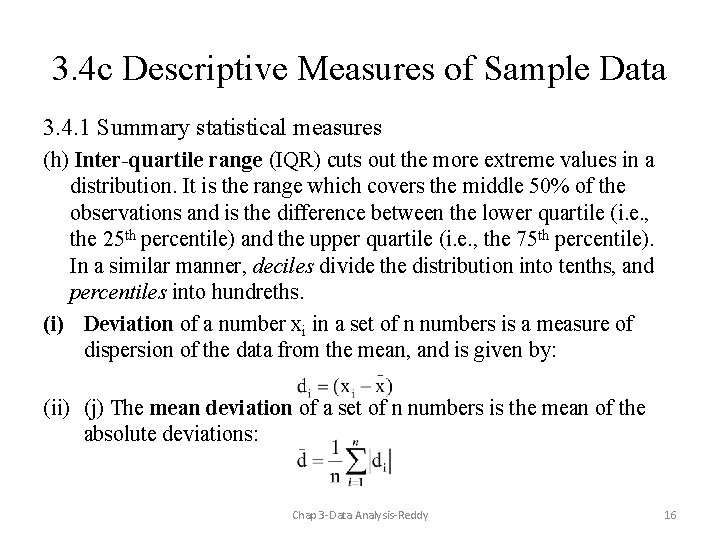
3. 4 c Descriptive Measures of Sample Data 3. 4. 1 Summary statistical measures (h) Inter-quartile range (IQR) cuts out the more extreme values in a distribution. It is the range which covers the middle 50% of the observations and is the difference between the lower quartile (i. e. , the 25 th percentile) and the upper quartile (i. e. , the 75 th percentile). In a similar manner, deciles divide the distribution into tenths, and percentiles into hundreths. (i) Deviation of a number xi in a set of n numbers is a measure of dispersion of the data from the mean, and is given by: (ii) (j) The mean deviation of a set of n numbers is the mean of the absolute deviations: Chap 3 -Data Analysis-Reddy 16

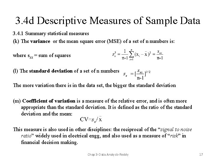
3. 4 d Descriptive Measures of Sample Data 3. 4. 1 Summary statistical measures (k) The variance or the mean square error (MSE) of a set of n numbers is: where sxx = sum of squares (l) The standard deviation of a set of n numbers The more variation there is in the data set, the bigger the standard deviation (m) Coefficient of variation is a measure of the relative error, and is often more appropriate than the standard deviation. It is defined as the ratio of the standard deviation and the mean: This measure is also used in other disciplines: the reciprocal of the “signal to noise ratio” widely used in electrical engg, and also used as a measure of “risk” in financial decision making. Chap 3 -Data Analysis-Reddy 17

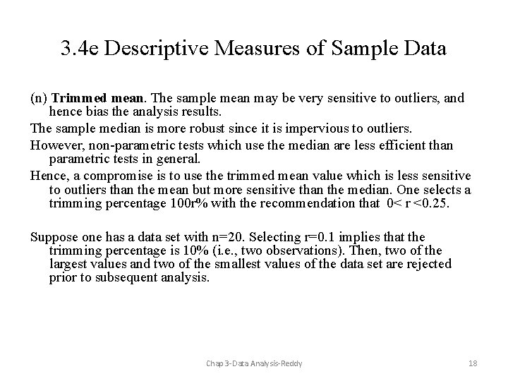
3. 4 e Descriptive Measures of Sample Data (n) Trimmed mean. The sample mean may be very sensitive to outliers, and hence bias the analysis results. The sample median is more robust since it is impervious to outliers. However, non-parametric tests which use the median are less efficient than parametric tests in general. Hence, a compromise is to use the trimmed mean value which is less sensitive to outliers than the mean but more sensitive than the median. One selects a trimming percentage 100 r% with the recommendation that 0< r <0. 25. Suppose one has a data set with n=20. Selecting r=0. 1 implies that the trimming percentage is 10% (i. e. , two observations). Then, two of the largest values and two of the smallest values of the data set are rejected prior to subsequent analysis. Chap 3 -Data Analysis-Reddy 18

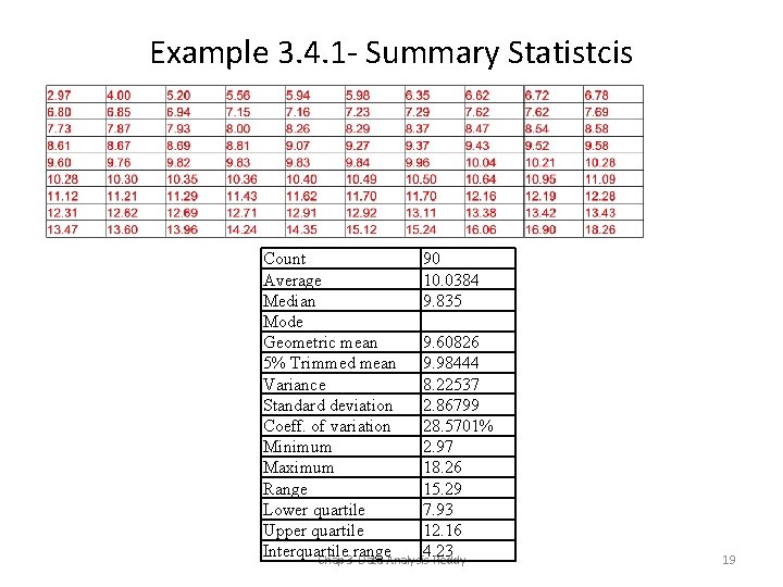
Example 3. 4. 1 - Summary Statistcis Count 90 Average 10. 0384 Median 9. 835 Mode Geometric mean 9. 60826 5% Trimmed mean 9. 98444 Variance 8. 22537 Standard deviation 2. 86799 Coeff. of variation 28. 5701% Minimum 2. 97 Maximum 18. 26 Range 15. 29 Lower quartile 7. 93 Upper quartile 12. 16 Interquartile range 4. 23 Chap 3 -Data Analysis-Reddy 19

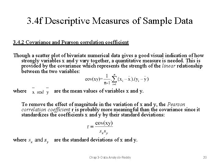
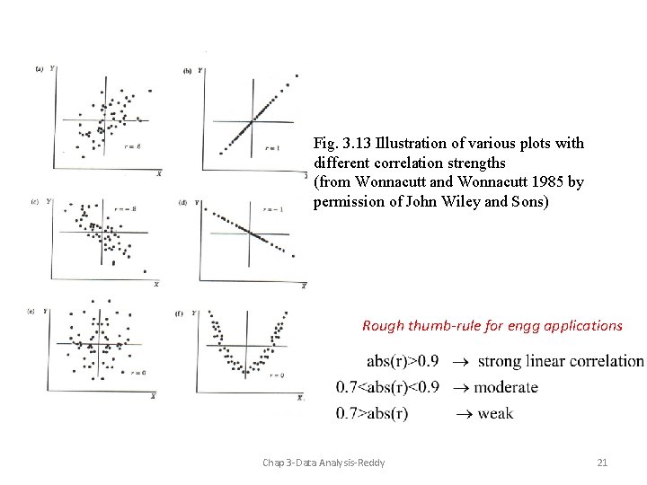
3. 4 f Descriptive Measures of Sample Data 3. 4. 2 Covariance and Pearson correlation coefficient Though a scatter plot of bivariate numerical data gives a good visual indication of how strongly variables x and y vary together, a quantitative measure is needed. This is provided by the covariance which represents the strength of the linear relationship between the two variables: where are the mean values of variables x and y. To remove the effect of magnitude in the variation of x and y, the Pearson correlation coefficient r is probably more meaningful than the covariance since it standardizes the coefficients x and y by their standard deviations: where are the standard deviations of x and y. Chap 3 -Data Analysis-Reddy 20

Fig. 3. 13 Illustration of various plots with different correlation strengths (from Wonnacutt and Wonnacutt 1985 by permission of John Wiley and Sons) Rough thumb-rule for engg applications Chap 3 -Data Analysis-Reddy 21

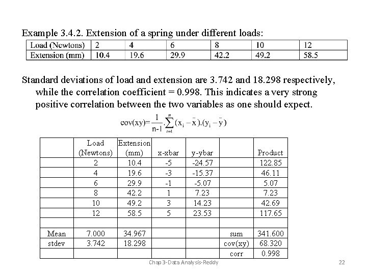
Example 3. 4. 2. Extension of a spring under different loads: Standard deviations of load and extension are 3. 742 and 18. 298 respectively, while the correlation coefficient = 0. 998. This indicates a very strong positive correlation between the two variables as one should expect. Load Extension (Newtons) (mm) x-xbar 2 10. 4 -5 4 19. 6 -3 6 29. 9 -1 8 42. 2 1 10 49. 2 3 12 58. 5 5 Mean stdev 7. 000 3. 742 y-ybar -24. 57 -15. 37 -5. 07 7. 23 14. 23 23. 53 34. 967 18. 298 Product 122. 85 46. 11 5. 07 7. 23 42. 69 117. 65 sum 341. 600 cov(xy) 68. 320 corr 0. 998 Chap 3 -Data Analysis-Reddy 22

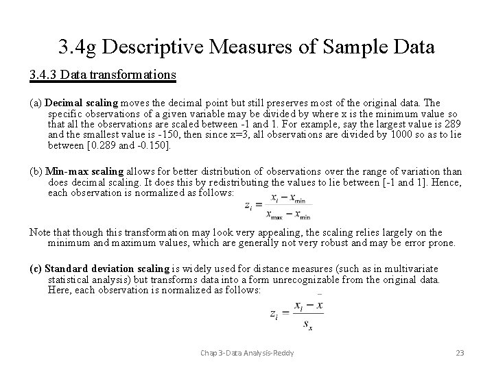
3. 4 g Descriptive Measures of Sample Data 3. 4. 3 Data transformations (a) Decimal scaling moves the decimal point but still preserves most of the original data. The specific observations of a given variable may be divided by where x is the minimum value so that all the observations are scaled between -1 and 1. For example, say the largest value is 289 and the smallest value is -150, then since x=3, all observations are divided by 1000 so as to lie between [0. 289 and -0. 150]. (b) Min-max scaling allows for better distribution of observations over the range of variation than does decimal scaling. It does this by redistributing the values to lie between [-1 and 1]. Hence, each observation is normalized as follows: Note that though this transformation may look very appealing, the scaling relies largely on the minimum and maximum values, which are generally not very robust and may be error prone. (c) Standard deviation scaling is widely used for distance measures (such as in multivariate statistical analysis) but transforms data into a form unrecognizable from the original data. Here, each observation is normalized as follows: Chap 3 -Data Analysis-Reddy 23

3. 5 a Plotting Data Graphical representations of data are the backbone of exploratory data analysis. they can serve as mediums to communicate information (what the author wishes to convey) not just to explore data trends They are usually limited to one-, two- and three-dimensional data. In the last few decades, there has been a dramatic increase in the types of graphical displays largely due to the seminal contributions of Tukey (1988), Cleveland (1985) and Tufte (1990, 2001). A particular graph is selected based on its ability to emphasize certain characteristics or behavior of 1 -D data, or to indicate relations between 2 - and 3 -dimension data. A simple manner of separating these characteristics is to view them as being: – cross-sectional (i. e. , the sequence in which the data has been collected is not retained), – time series data, – hybrid or combined, and – relational (i. e. , emphasizing the joint variation of two or more variables). Chap 3 -Data Analysis-Reddy 24

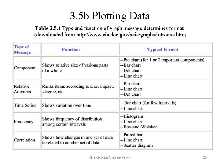
3. 5 b Plotting Data Table 3. 5. 1 Type and function of graph message determines format (downloaded from http: //www. eia. doe. gov/neic/graphs/introduc. htm) Chap 3 -Data Analysis-Reddy 25

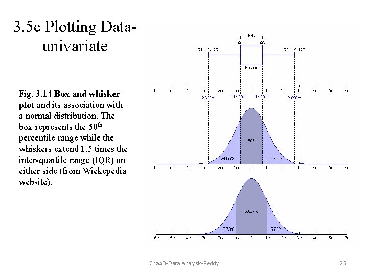
3. 5 c Plotting Dataunivariate Fig. 3. 14 Box and whisker plot and its association with a normal distribution. The box represents the 50 th percentile range while the whiskers extend 1. 5 times the inter-quartile range (IQR) on either side (from Wickepedia website). Chap 3 -Data Analysis-Reddy 26

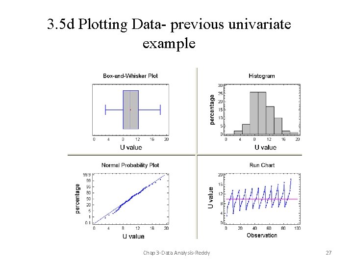
3. 5 d Plotting Data- previous univariate example Chap 3 -Data Analysis-Reddy 27

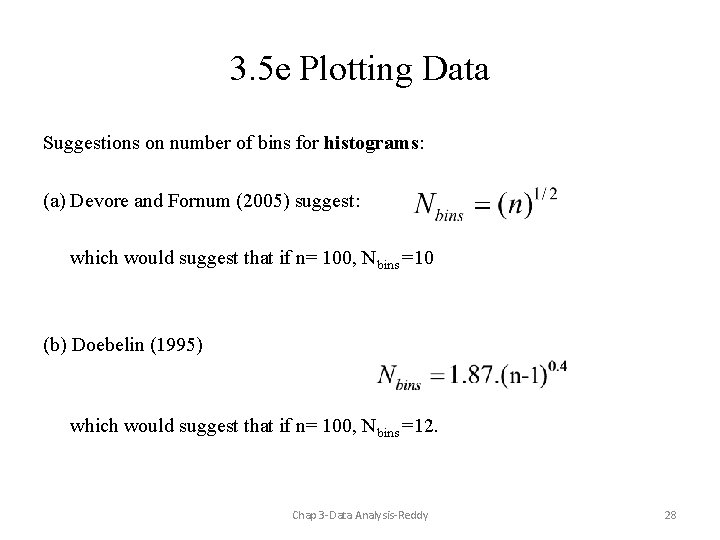
3. 5 e Plotting Data Suggestions on number of bins for histograms: (a) Devore and Fornum (2005) suggest: which would suggest that if n= 100, Nbins =10 (b) Doebelin (1995) which would suggest that if n= 100, Nbins =12. Chap 3 -Data Analysis-Reddy 28

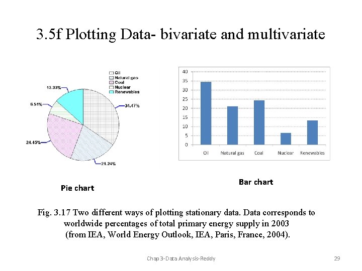
3. 5 f Plotting Data- bivariate and multivariate Bar chart Pie chart Fig. 3. 17 Two different ways of plotting stationary data. Data corresponds to worldwide percentages of total primary energy supply in 2003 (from IEA, World Energy Outlook, IEA, Paris, France, 2004). Chap 3 -Data Analysis-Reddy 29

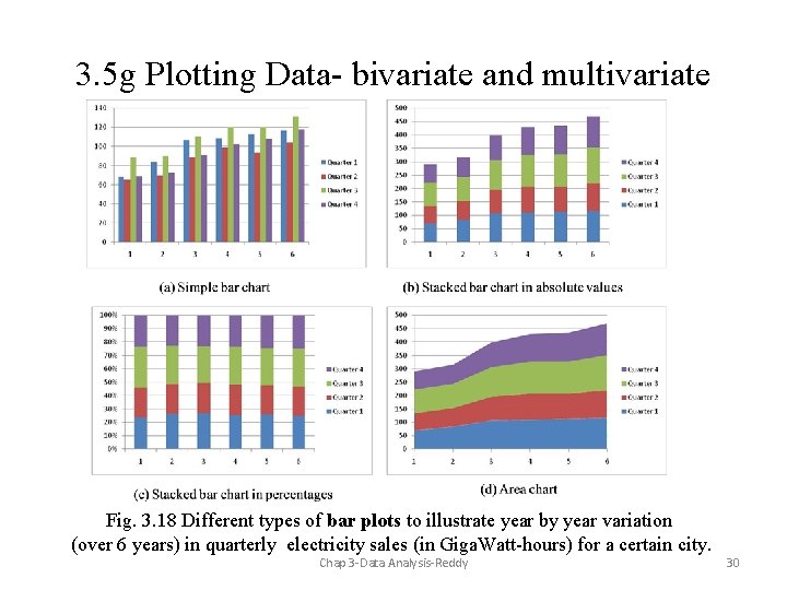
3. 5 g Plotting Data- bivariate and multivariate Fig. 3. 18 Different types of bar plots to illustrate year by year variation (over 6 years) in quarterly electricity sales (in Giga. Watt-hours) for a certain city. Chap 3 -Data Analysis-Reddy 30

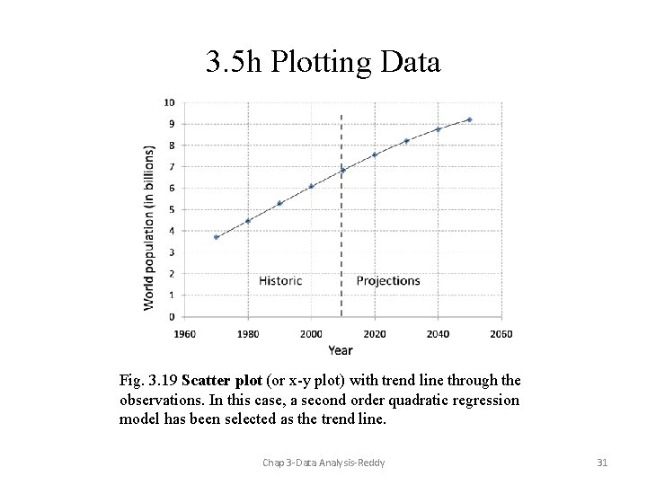
3. 5 h Plotting Data Fig. 3. 19 Scatter plot (or x-y plot) with trend line through the observations. In this case, a second order quadratic regression model has been selected as the trend line. Chap 3 -Data Analysis-Reddy 31

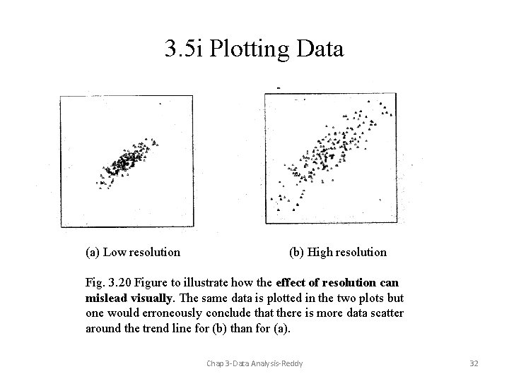
3. 5 i Plotting Data (a) Low resolution (b) High resolution Fig. 3. 20 Figure to illustrate how the effect of resolution can mislead visually. The same data is plotted in the two plots but one would erroneously conclude that there is more data scatter around the trend line for (b) than for (a). Chap 3 -Data Analysis-Reddy 32

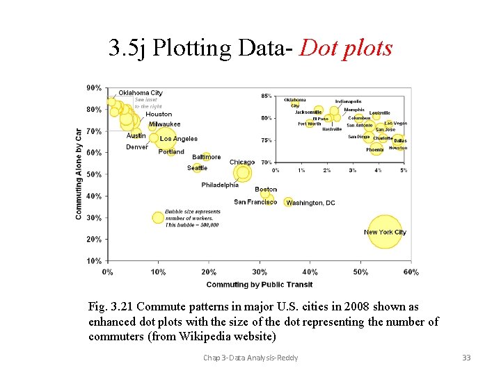
3. 5 j Plotting Data- Dot plots Fig. 3. 21 Commute patterns in major U. S. cities in 2008 shown as enhanced dot plots with the size of the dot representing the number of commuters (from Wikipedia website) Chap 3 -Data Analysis-Reddy 33

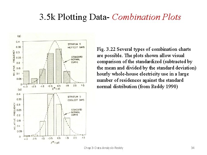
3. 5 k Plotting Data- Combination Plots Fig. 3. 22 Several types of combination charts are possible. The plots shown allow visual comparison of the standardized (subtracted by the mean and divided by the standard deviation) hourly whole-house electricity use in a large number of residences against the standard normal distribution (from Reddy 1990) Chap 3 -Data Analysis-Reddy 34

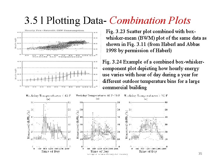
3. 5 l Plotting Data- Combination Plots Fig. 3. 23 Scatter plot combined with boxwhisker-mean (BWM) plot of the same data as shown in Fig. 3. 11 (from Haberl and Abbas 1998 by permission of Haberl) Fig. 3. 24 Example of a combined box-whiskercomponent plot depicting how hourly energy use varies with hour of day during a year for different outdoor temperature bins for a large commercial building Chap 3 -Data Analysis-Reddy 35

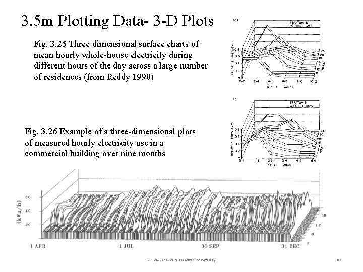
3. 5 m Plotting Data- 3 -D Plots Fig. 3. 25 Three dimensional surface charts of mean hourly whole-house electricity during different hours of the day across a large number of residences (from Reddy 1990) Fig. 3. 26 Example of a three-dimensional plots of measured hourly electricity use in a commercial building over nine months Chap 3 -Data Analysis-Reddy 36

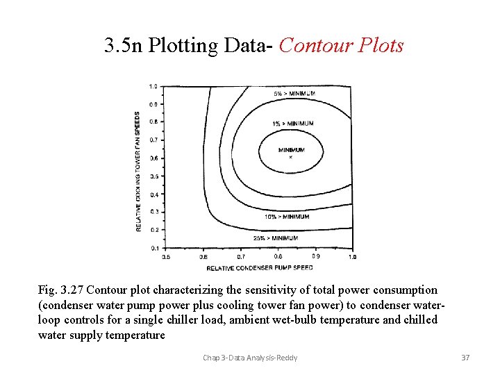
3. 5 n Plotting Data- Contour Plots Fig. 3. 27 Contour plot characterizing the sensitivity of total power consumption (condenser water pump power plus cooling tower fan power) to condenser waterloop controls for a single chiller load, ambient wet-bulb temperature and chilled water supply temperature Chap 3 -Data Analysis-Reddy 37

3. 5 o Plotting Data- Carpet Plots Fig. 3. 29 Scatter plot matrix or carpet plots for multivariable graphical data analysis. The data corresponds to hourly climatic data for Phoenix, AZ for January 1990. The bottom left hand corner frame indicates how solar radiation in Btu/hr-ft 2 (x-axis) varies with drybulb temperature (in 0 F) and is a flipped and rotated image of that at the top right hand corner. The HR variable represents humidity ratio (in lbm/lba). Points which fall distinctively outside the general scatter can be flagged as outliers. Chap 3 -Data Analysis-Reddy 38

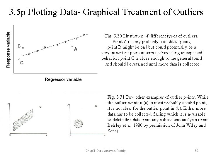
3. 5 p Plotting Data- Graphical Treatment of Outliers Fig. 3. 30 Illustration of different types of outliers. Point A is very probably a doubtful point; point B might be bad but could potentially be a very important point in terms of revealing unexpected behavior; point C is close enough to the general trend and should be retained until more data is collected Fig. 3. 31 Two other examples of outlier points. While the outlier point in (a) is most probably a valid point, it is not clear for the outlier point in (b). Either more data has to be collected, failing which it is advisable to delete this data from any subsequent analysis (from Belsley et al. 1980 by permission of John Wiley and Sons). Chap 3 -Data Analysis-Reddy 39

3. 6 Overall Measurement Uncertainty The International Organization of Standardization (ISO) and six other organizations have published guides which have established the experimental uncertainty standard (an example is ANSI/ASME, 1990). 3. 6. 1 Need for uncertainty analysis Any measurement exhibits some difference between the measured value and the true value and, therefore, has an associated uncertainty. A statement of measured value without an accompanying uncertainty statement has limited meaning. Uncertainty is the interval around the measured value within which the true value is expected to fall with some stated confidence level. “Good data” does not describe data that yields the desired answer. It describes data that yields a result within an acceptable uncertainty interval or, in other words, provides the acceptable degree of confidence in the result. Chap 3 -Data Analysis-Reddy 40

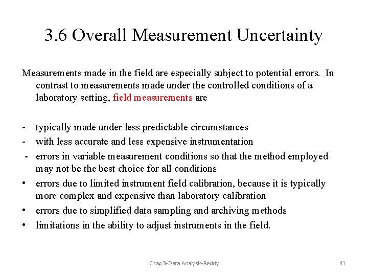
3. 6 Overall Measurement Uncertainty Measurements made in the field are especially subject to potential errors. In contrast to measurements made under the controlled conditions of a laboratory setting, field measurements are - typically made under less predictable circumstances - with less accurate and less expensive instrumentation - errors in variable measurement conditions so that the method employed may not be the best choice for all conditions • errors due to limited instrument field calibration, because it is typically more complex and expensive than laboratory calibration • errors due to simplified data sampling and archiving methods • limitations in the ability to adjust instruments in the field. Chap 3 -Data Analysis-Reddy 41

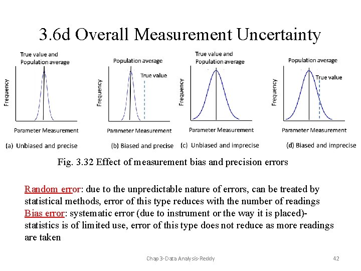
3. 6 d Overall Measurement Uncertainty Fig. 3. 32 Effect of measurement bias and precision errors Random error: due to the unpredictable nature of errors, can be treated by statistical methods, error of this type reduces with the number of readings Bias error: systematic error (due to instrument or the way it is placed)statistics is of limited use, error of this type does not reduce as more readings are taken Chap 3 -Data Analysis-Reddy 42

3. 6. 3 Random Uncertainty • UNCERTAINTY: interval around the measured value within which the true value is expected to fall at some confidence interval • For example, the statement that the measurement is within 5. 1 - 8. 2 at 95% implies that the probability of the actual value being between {5. 1, 8. 2} is 95% • A higher confidence interval would result in a wider range and vice versa • Usual confidence levels (CL) used are: 99%, 95% and 90%. • Significance level is also used: - for two-tailed distribution, 95% CL is the same as 0. 025 significance level Chap 3 -Data Analysis-Reddy 43

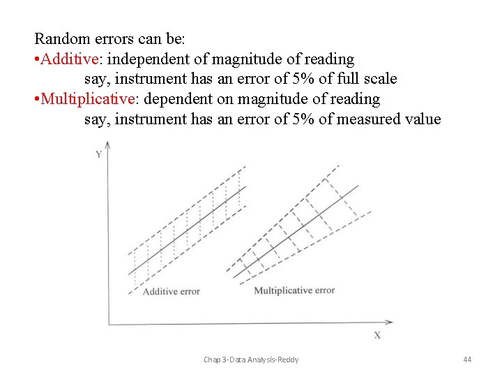
Random errors can be: • Additive: independent of magnitude of reading say, instrument has an error of 5% of full scale • Multiplicative: dependent on magnitude of reading say, instrument has an error of 5% of measured value Chap 3 -Data Analysis-Reddy 44

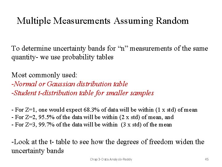
Multiple Measurements Assuming Random To determine uncertainty bands for “n” measurements of the same quantity- we use probability tables Most commonly used: -Normal or Gaussian distribution table -Student t-distribution table for smaller samples - For Z=1, one would expect 68. 3% of data will be within (1 x std) of mean - For Z=2, 95. 5% of the data will be within (2 x std) of mean, and - For Z=3, 99. 7% of the data will be within (3 x std) of the mean -Look at the t- table to see how the degrees of freedom widen the uncertainty bands Chap 3 -Data Analysis-Reddy 45

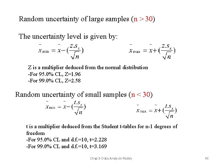
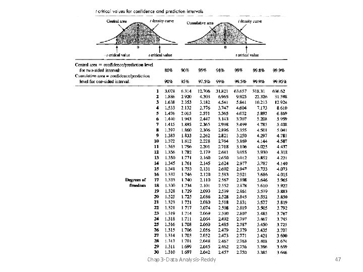
Random uncertainty of large samples (n > 30) The uncertainty level is given by: Z is a multiplier deduced from the normal distribution -For 95. 0% CL, Z=1. 96 -For 99. 0% CL, Z=2. 58 Random uncertainty of small samples (n < 30) t is a multiplier deduced from the Student t-tables for n-1 degrees of freedom -For 95. 0% CL and d. f. =10, t=2. 228 -For 99. 0% CL and d. f. =10, t=3. 169 Chap 3 -Data Analysis-Reddy 46

Chap 3 -Data Analysis-Reddy 47

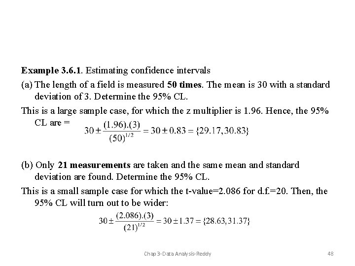
Example 3. 6. 1. Estimating confidence intervals (a) The length of a field is measured 50 times. The mean is 30 with a standard deviation of 3. Determine the 95% CL. This is a large sample case, for which the z multiplier is 1. 96. Hence, the 95% CL are = (b) Only 21 measurements are taken and the same mean and standard deviation are found. Determine the 95% CL. This is a small sample case for which the t-value=2. 086 for d. f. =20. Then, the 95% CL will turn out to be wider: Chap 3 -Data Analysis-Reddy 48

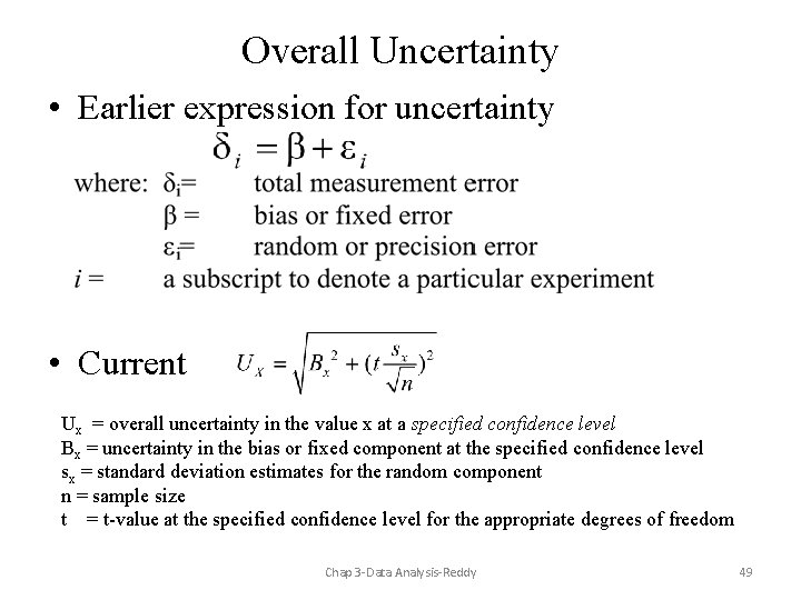
Overall Uncertainty • Earlier expression for uncertainty • Current Ux = overall uncertainty in the value x at a specified confidence level Bx = uncertainty in the bias or fixed component at the specified confidence level sx = standard deviation estimates for the random component n = sample size t = t-value at the specified confidence level for the appropriate degrees of freedom Chap 3 -Data Analysis-Reddy 49

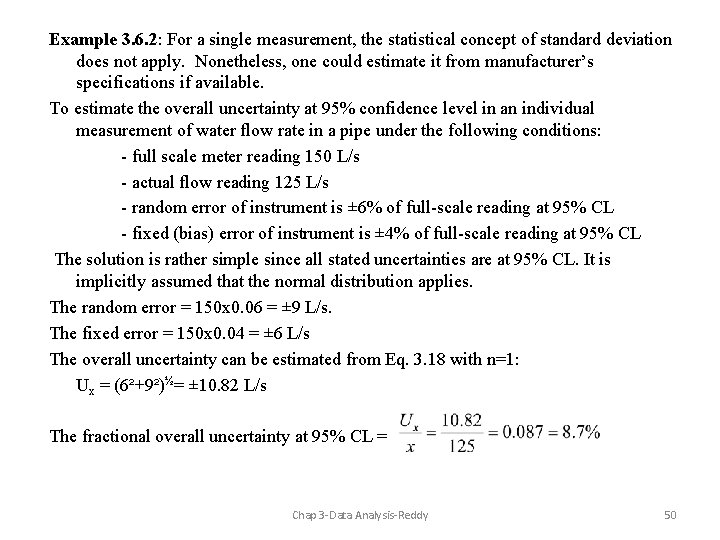
Example 3. 6. 2: For a single measurement, the statistical concept of standard deviation does not apply. Nonetheless, one could estimate it from manufacturer’s specifications if available. To estimate the overall uncertainty at 95% confidence level in an individual measurement of water flow rate in a pipe under the following conditions: - full scale meter reading 150 L/s - actual flow reading 125 L/s - random error of instrument is ± 6% of full-scale reading at 95% CL - fixed (bias) error of instrument is ± 4% of full-scale reading at 95% CL The solution is rather simple since all stated uncertainties are at 95% CL. It is implicitly assumed that the normal distribution applies. The random error = 150 x 0. 06 = ± 9 L/s. The fixed error = 150 x 0. 04 = ± 6 L/s The overall uncertainty can be estimated from Eq. 3. 18 with n=1: Ux = (6²+9²)½= ± 10. 82 L/s The fractional overall uncertainty at 95% CL = Chap 3 -Data Analysis-Reddy 50

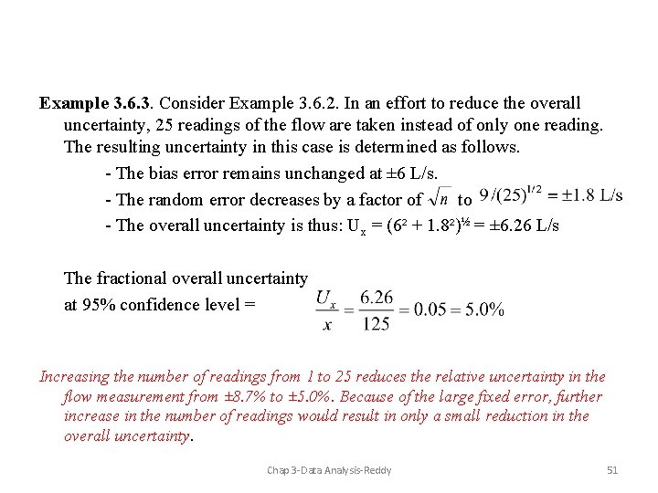
Example 3. 6. 3. Consider Example 3. 6. 2. In an effort to reduce the overall uncertainty, 25 readings of the flow are taken instead of only one reading. The resulting uncertainty in this case is determined as follows. - The bias error remains unchanged at ± 6 L/s. - The random error decreases by a factor of to - The overall uncertainty is thus: Ux = (6² + 1. 8²)½ = ± 6. 26 L/s The fractional overall uncertainty at 95% confidence level = Increasing the number of readings from 1 to 25 reduces the relative uncertainty in the flow measurement from ± 8. 7% to ± 5. 0%. Because of the large fixed error, further increase in the number of readings would result in only a small reduction in the overall uncertainty. Chap 3 -Data Analysis-Reddy 51

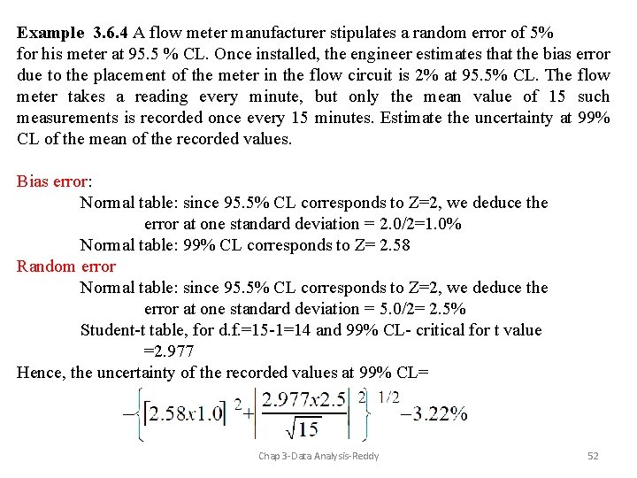
Example 3. 6. 4 A flow meter manufacturer stipulates a random error of 5% for his meter at 95. 5 % CL. Once installed, the engineer estimates that the bias error due to the placement of the meter in the flow circuit is 2% at 95. 5% CL. The flow meter takes a reading every minute, but only the mean value of 15 such measurements is recorded once every 15 minutes. Estimate the uncertainty at 99% CL of the mean of the recorded values. Bias error: Normal table: since 95. 5% CL corresponds to Z=2, we deduce the error at one standard deviation = 2. 0/2=1. 0% Normal table: 99% CL corresponds to Z= 2. 58 Random error Normal table: since 95. 5% CL corresponds to Z=2, we deduce the error at one standard deviation = 5. 0/2= 2. 5% Student-t table, for d. f. =15 -1=14 and 99% CL- critical for t value =2. 977 Hence, the uncertainty of the recorded values at 99% CL= Chap 3 -Data Analysis-Reddy 52

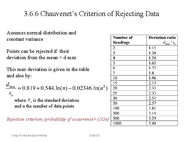
3. 6. 6 Chauvenet’s Criterion of Rejecting Data Assumes normal distribution and constant variance Points can be rejected if their deviation from the mean > d max This max deviation is given in the table and also by: where is the standard deviation and n the number of data points Rejection criterion: probability of occurrence> (1/2 n) Chap 3 -Data Analysis-Reddy Slide 53

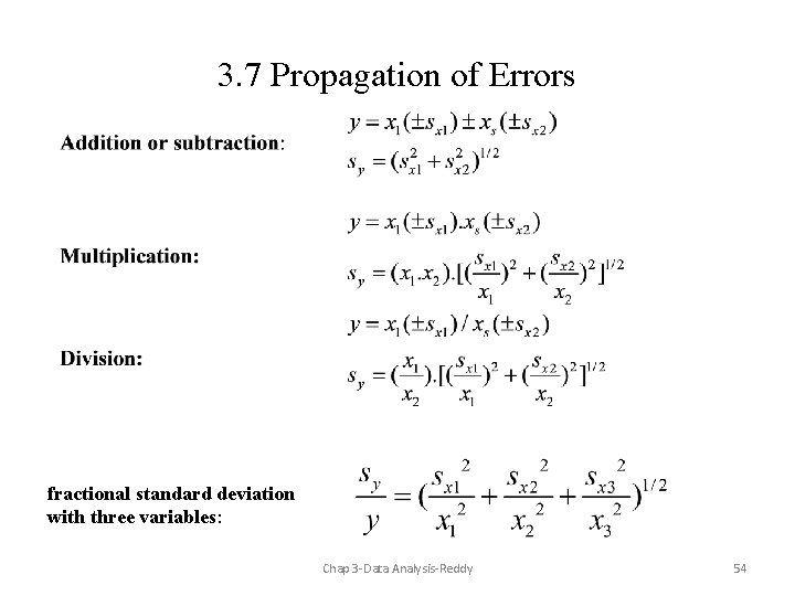
3. 7 Propagation of Errors fractional standard deviation with three variables: Chap 3 -Data Analysis-Reddy 54

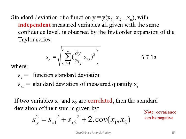
Standard deviation of a function y = y(x 1, x 2, . . , xn), with independent measured variables all given with the same confidence level, is obtained by the first order expansion of the Taylor series: 3. 7. 1 a where: sy = function standard deviation sx, i = standard deviation of measured quantity xi If two variables x 1 and x 2 are correlated, then the standard deviation of their sum is given by: Note: covariance can be negative Chap 3 -Data Analysis-Reddy 55

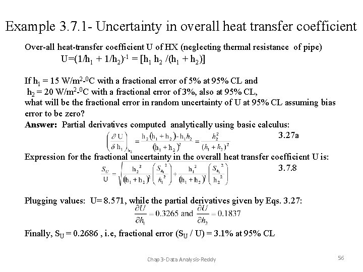
Example 3. 7. 1 - Uncertainty in overall heat transfer coefficient Over-all heat-transfer coefficient U of HX (neglecting thermal resistance of pipe) U=(1/h 1 + 1/h 2)-1 = [h 1 h 2 /(h 1 + h 2)] If h 1 = 15 W/m 2 -0 C with a fractional error of 5% at 95% CL and h 2 = 20 W/m 2 -0 C with a fractional error of 3%, also at 95% CL, what will be the fractional error in random uncertainty of U at 95% CL assuming bias error to be zero? Answer: Partial derivatives computed analytically using basic calculus: 3. 27 a Expression for the fractional uncertainty in the overall heat transfer coefficient U is: 3. 7. 8 Plugging values: U= 8. 571, while the partial derivatives given by Eqs. 3. 27: Finally, SU = 0. 2686 , i. e, fractional error (SU / U) = 3. 1% at 95% CL Chap 3 -Data Analysis-Reddy 56

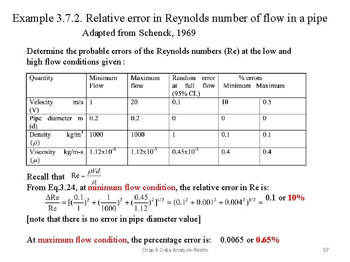
Example 3. 7. 2. Relative error in Reynolds number of flow in a pipe Adapted from Schenck, 1969 Determine the probable errors of the Reynolds numbers (Re) at the low and high flow conditions given : Recall that From Eq. 3. 24, at minimum flow condition, the relative error in Re is: 0. 1 or 10% [note that there is no error in pipe diameter value] At maximum flow condition, the percentage error is: Chap 3 -Data Analysis-Reddy 0. 0065 or 0. 65% 57

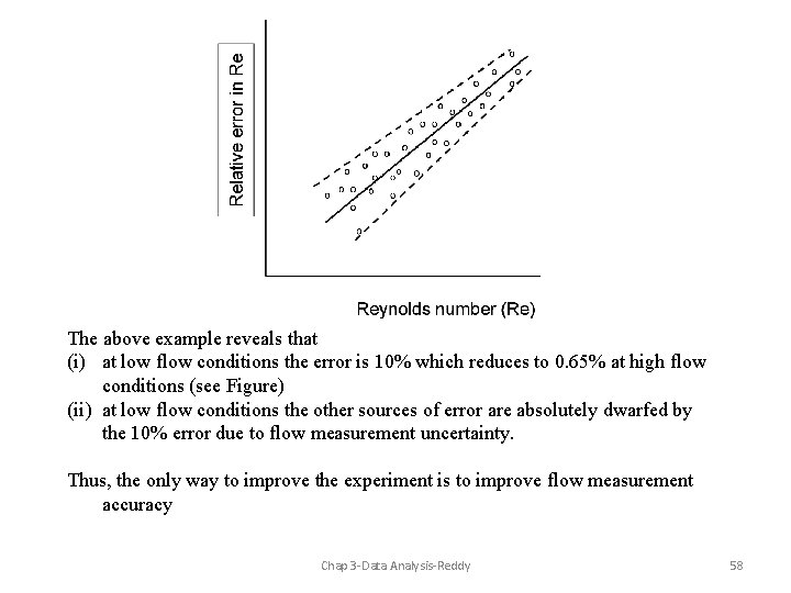
The above example reveals that (i) at low flow conditions the error is 10% which reduces to 0. 65% at high flow conditions (see Figure) (ii) at low flow conditions the other sources of error are absolutely dwarfed by the 10% error due to flow measurement uncertainty. Thus, the only way to improve the experiment is to improve flow measurement accuracy Chap 3 -Data Analysis-Reddy 58

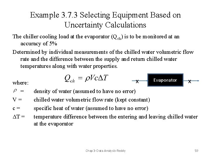
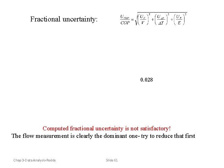
Example 3. 7. 3 Selecting Equipment Based on Uncertainty Calculations The chiller cooling load at the evaporator (Qch) is to be monitored at an accuracy of 5% Determined by individual measurements of the chilled water volumetric flow rate and the difference between the supply and return chilled water temperatures along with water properties. where: = V= c= ΔT = x Evaporator x density of water (assumed to have no error) chilled water volumetric flow rate (kept constant) specific heat of water (assumed to have no error) temperature difference between the entering and leaving chilled water at the evaporator Chap 3 -Data Analysis-Reddy 59

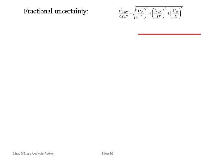
Fractional uncertainty: Chap 3 -Data Analysis-Reddy Slide 60

Fractional uncertainty: 0. 028 28 Computed fractional uncertainty is not satisfactory! The flow measurement is clearly the dominant one- try to reduce that first Chap 3 -Data Analysis-Reddy Slide 61

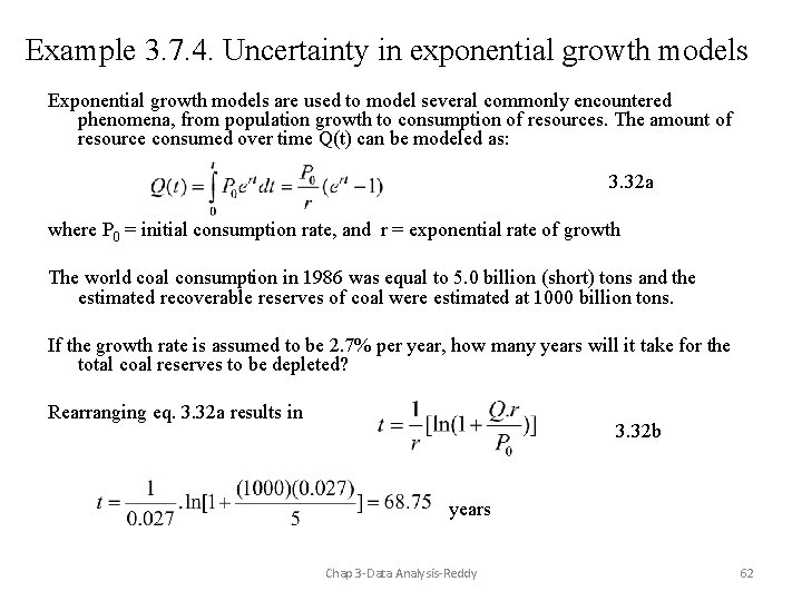
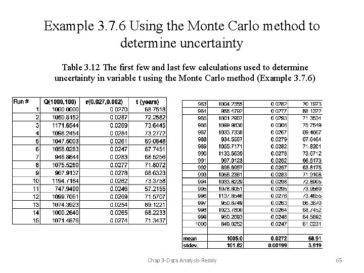
Example 3. 7. 4. Uncertainty in exponential growth models Exponential growth models are used to model several commonly encountered phenomena, from population growth to consumption of resources. The amount of resource consumed over time Q(t) can be modeled as: 3. 32 a where P 0 = initial consumption rate, and r = exponential rate of growth The world coal consumption in 1986 was equal to 5. 0 billion (short) tons and the estimated recoverable reserves of coal were estimated at 1000 billion tons. If the growth rate is assumed to be 2. 7% per year, how many years will it take for the total coal reserves to be depleted? Rearranging eq. 3. 32 a results in 3. 32 b years Chap 3 -Data Analysis-Reddy 62

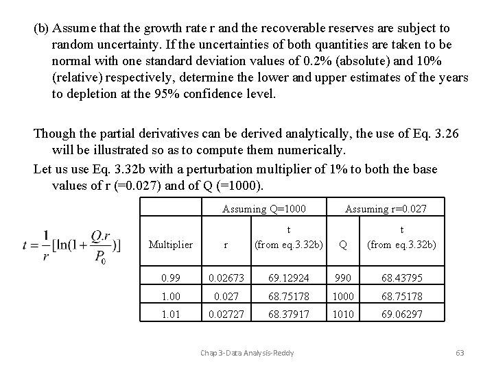
(b) Assume that the growth rate r and the recoverable reserves are subject to random uncertainty. If the uncertainties of both quantities are taken to be normal with one standard deviation values of 0. 2% (absolute) and 10% (relative) respectively, determine the lower and upper estimates of the years to depletion at the 95% confidence level. Though the partial derivatives can be derived analytically, the use of Eq. 3. 26 will be illustrated so as to compute them numerically. Let us use Eq. 3. 32 b with a perturbation multiplier of 1% to both the base values of r (=0. 027) and of Q (=1000). Assuming Q=1000 Assuming r=0. 027 Multiplier r t (from eq. 3. 32 b) 0. 99 0. 02673 69. 12924 990 68. 43795 1. 00 0. 027 68. 75178 1000 68. 75178 1. 01 0. 02727 68. 37917 1010 69. 06297 Chap 3 -Data Analysis-Reddy Q t (from eq. 3. 32 b) 63

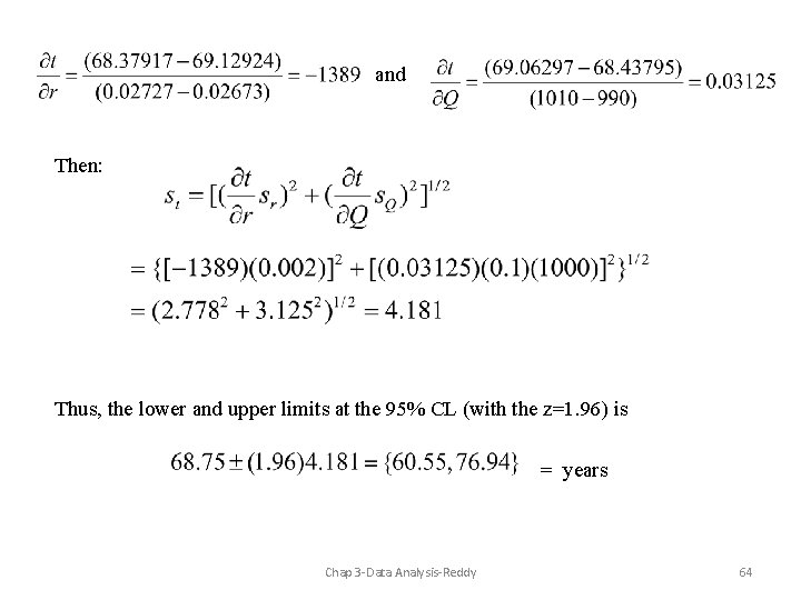
and Then: Thus, the lower and upper limits at the 95% CL (with the z=1. 96) is = years Chap 3 -Data Analysis-Reddy 64

Example 3. 7. 6 Using the Monte Carlo method to determine uncertainty Table 3. 12 The first few and last few calculations used to determine uncertainty in variable t using the Monte Carlo method (Example 3. 7. 6) Chap 3 -Data Analysis-Reddy 65

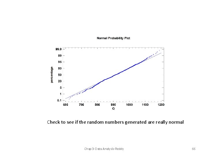
Check to see if the random numbers generated are really normal Chap 3 -Data Analysis-Reddy 66

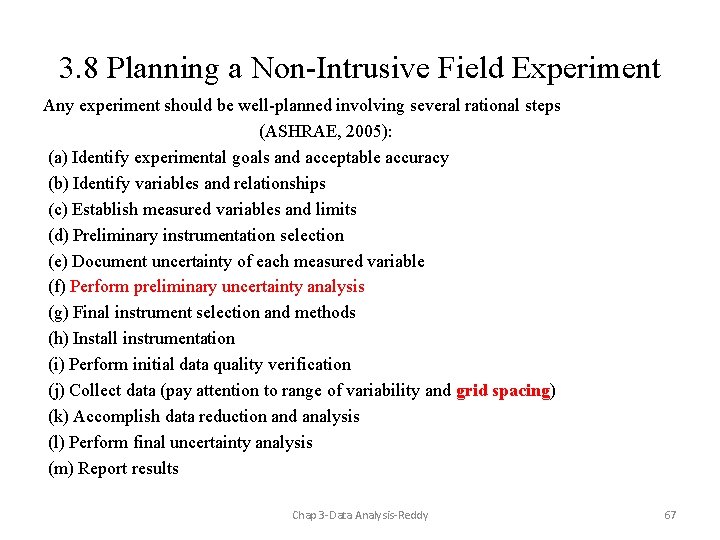
3. 8 Planning a Non-Intrusive Field Experiment Any experiment should be well-planned involving several rational steps (ASHRAE, 2005): (a) Identify experimental goals and acceptable accuracy (b) Identify variables and relationships (c) Establish measured variables and limits (d) Preliminary instrumentation selection (e) Document uncertainty of each measured variable (f) Perform preliminary uncertainty analysis (g) Final instrument selection and methods (h) Install instrumentation (i) Perform initial data quality verification (j) Collect data (pay attention to range of variability and grid spacing) (k) Accomplish data reduction and analysis (l) Perform final uncertainty analysis (m) Report results Chap 3 -Data Analysis-Reddy 67

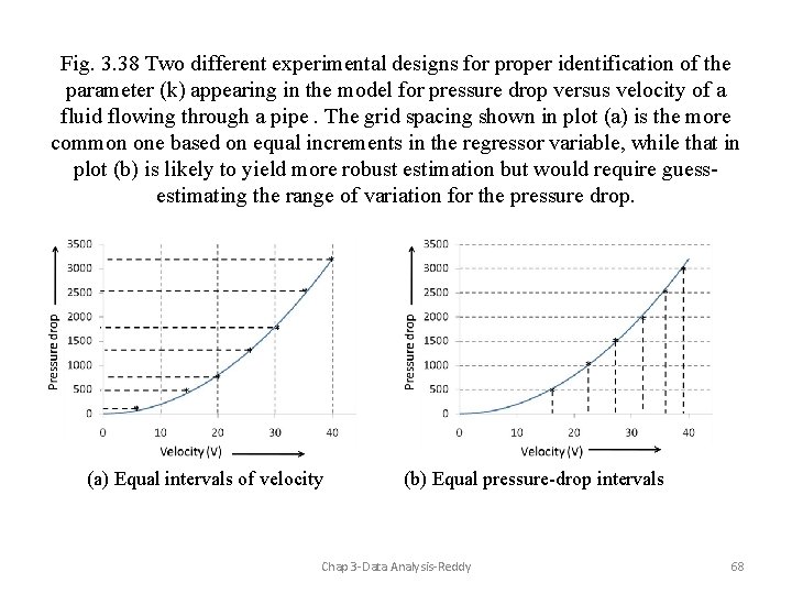
Fig. 3. 38 Two different experimental designs for proper identification of the parameter (k) appearing in the model for pressure drop versus velocity of a fluid flowing through a pipe. The grid spacing shown in plot (a) is the more common one based on equal increments in the regressor variable, while that in plot (b) is likely to yield more robust estimation but would require guessestimating the range of variation for the pressure drop. (a) Equal intervals of velocity (b) Equal pressure-drop intervals Chap 3 -Data Analysis-Reddy 68