Chapter 3 Data Analysis in Consumer Theory 132022

Chapter 3: Data Analysis in Consumer Theory 1/3/2022 1

Introduction: • This chapter shows you how can we study the impact of one variable on another in isolation from other factors which are also deemed to be important? • Economists use a technique called Regression Analysis. • Regression analysis is two types, simple regression, which looks at the statistical relationship between two variables, one dependent on another, however in the multiple regression there is a relation between one dependent variable and many independent variables. 1/3/2022 2

2. Theoretical explorations • We will use an example based on research done by the Indian economist and statistician Krishnaji (1992). • On this example we will estimate the effect of (the relation between) changes in the price of cereals (basic food items such as wheat) as independent variable on (and) the demand for basic manufactured consumer goods (clothing, and so on) as dependent variable. We will estimate this relationship through studying the effects of income and substitutions of the goods. 2. 1 Income and substitution effects on the consumption: • We assume that the price of cereals run up, in such case there are two possible effects of a rise in the price of cereals: • 1. A substitution effect: as cereals become expensive relative to other goods, consumers will switch their consumption to other goods. • 2. An income effect: consumers will have less real income to spend. If cereals are a normal good, the consumption of cereals will fall as a result. If cereals are an inferior good, the income effect of a rise in the price will increase cereals consumption. 1/3/2022 3

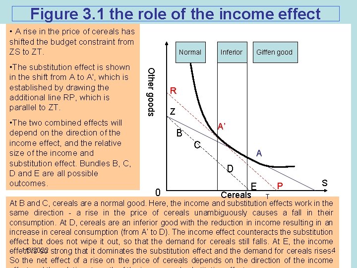
Figure 3. 1 the role of the income effect • A rise in the price of cereals has shifted the budget constraint from ZS to ZT. • The two combined effects will depend on the direction of the income effect, and the relative size of the income and substitution effect. Bundles B, C, D and E are all possible outcomes. Other goods • The substitution effect is shown in the shift from A to A', which is established by drawing the additional line RP, which is parallel to ZT. Normal Inferior Giffen good R Z A’ B C A D 0 P E Cereals T S At B and C, cereals are a normal good. Here, the income and substitution effects work in the same direction - a rise in the price of cereals unambiguously causes a fall in their consumption. At D, cereals are an inferior good with the reduction in income resulting in an increase in cereal consumption (from A’ to D). The income effect counteracts the substitution effect but does not wipe it out, so that the demand for cereals still falls. At E, the income 1/3/2022 effect is so strong that it dominates the substitution effect and the demand for cereals rises. 4 So the net effect of a rise on the price of cereals depends on the direction of the income

• Putting the income and Substitution effects together we can see that for the poor, a weak substitution effect is likely to be outweighed by a strong income effect. So the net effect of a rise in the price of cereals is a fall in the demand for manufactured consumer goods, and we might expect the total effect to be quite strong. • For the rich, however, the relative strengths of the two effects may be reversed. The income effect will be smaller and the substitution effect larger, therefore the effect of the price of cereals is more likely to be a (possibly small) rise in the consumption of manufactured consumer goods. • Here the Krishnaji's hypothesis which is, if the price of cereals increases, then, other things being equal, the demand for manufactures will fall as poor consumers are forced to reduce their consumption of manufactures. This assumption will find support from consumer theory. since in India, where the poor vastly outnumber the rich. 1/3/2022 5

3. Modelling data: How can we translate a theoretical idea into a statistical model for empirical investigation. 3. 1 The variables in play: • • Dependent variable: is the one the model claims is determined by the other variables. • Independent variable (explanatory) like here the price of cereals. But, obviously, the price of cereals is not the only explanatory variable that matters. At the very least we should also take account of two additional explanatory variables, namely, personal disposable income and the price of manufactured consumer goods. • Therefore, here in the example, we will have four variables: one dependent variable and three explanatory variables as following: The Data: Dm the demand for manufactured consumer goods Px a the price of manufactured goods Pc the price of cereals y personal disposable income 1/3/2022 6

• We should have the data for these four variables, for example, we will have a data of the independent variable, Dm, measures per capita : expenditure on manufactured consumer goods at constant 1970 -1 prices. • This means the expenditure in each year is evaluated using the 1970 -1 base year prices for manufactured goods. This gives a measure of the real quantity of manufactured consumer goods purchased. • Saying that our variable is per capita means that the total demand is divided by the population, so that Dm measures the real quantity of manufactured consumer goods sold per head of population in India. 3. 2 The components of a statistical model: • A statistical model, can always be depicted as: Model = Structure + Noise. • 'structure' refers to the structural patterns in the data - the sound - and 'noise' (the error or disturbance term ) contains a multitude of small uncontrollable factors that interfere with this basic structure. • In empirical economics, if we fail to model one or more important feature in the data, the noise component may blur the message we receive. • In regression analysis, if we leave out an important explanatory variable, we are unlikely to get a clear message from the data. 1/3/2022 7

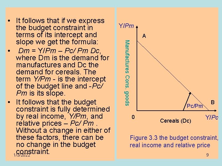
3. 3 Modelling Krishnaji's hypothesis: • in order to investigate Krishnaji's hypothesis we will write the relation between the dependent variable and the explanatory variables, on the one hand, and the error term, on the other, as a mathematical expression. Relative prices and real income: • In demand analysis it is customary to model the demand for a commodity as a function of relative prices rather than absolute prices, and of real income rather than disposable income per capita. Figure 3. 3 shows the budget constraint which is determined by the consumer's income and the two prices. 1/3/2022 8

Y/Pm A Manufactures Cons. goods • It follows that if we express the budget constraint in terms of its intercept and slope we get the formula: • Dm = Y/Pm – Pc/ Pm Dc, where Dm is the demand for manufactures and Dc the demand for cereals. The term Y/Pm - is the intercept of the budget line and -Pc/ Pm is its slope. • It follows that the budget constraint is fully determined by real income, Y/Pm, and relative prices – Pc/ Pm. Without a change in either of these factors, there can be no change in the budget constraint. 1/3/2022 B Pc/Pm 0 Cereals (Dc) Y/Pc Figure 3. 3 the budget constraint, real income and relative price 9

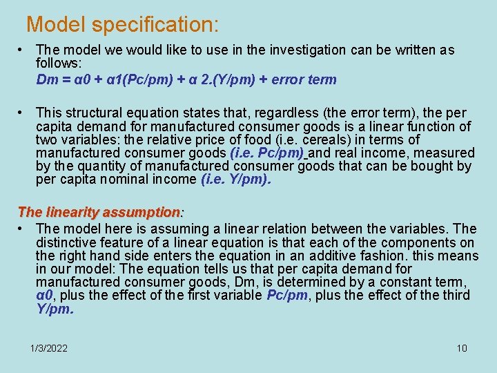
Model specification: • The model we would like to use in the investigation can be written as follows: Dm = α 0 + α 1(Pc/pm) + α 2. (Y/pm) + error term • This structural equation states that, regardless (the error term), the per capita demand for manufactured consumer goods is a linear function of two variables: the relative price of food (i. e. cereals) in terms of manufactured consumer goods (i. e. Pc/pm) and real income, measured by the quantity of manufactured consumer goods that can be bought by per capita nominal income (i. e. Y/pm). The linearity assumption: • The model here is assuming a linear relation between the variables. The distinctive feature of a linear equation is that each of the components on the right hand side enters the equation in an additive fashion. this means in our model: The equation tells us that per capita demand for manufactured consumer goods, Dm, is determined by a constant term, α 0, plus the effect of the first variable Pc/pm, plus the effect of the third Y/pm. 1/3/2022 10

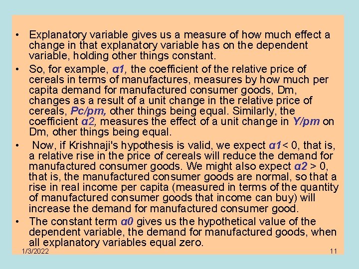
• Explanatory variable gives us a measure of how much effect a change in that explanatory variable has on the dependent variable, holding other things constant. • So, for example, α 1, the coefficient of the relative price of cereals in terms of manufactures, measures by how much per capita demand for manufactured consumer goods, Dm, changes as a result of a unit change in the relative price of cereals, Pc/pm, other things being equal. Similarly, the coefficient α 2, measures the effect of a unit change in Y/pm on Dm, other things being equal. • Now, if Krishnaji's hypothesis is valid, we expect α 1< 0, that is, a relative rise in the price of cereals will reduce the demand for manufactured consumer goods. We might also expect α 2 > 0, that is, the manufactured consumer goods are normal, so that a rise in real income per capita (measured in terms of the quantity of manufactured consumer goods that income can buy) will increase the demand for manufactured consumer good. • The constant term α 0 gives us the hypothetical value of the dependent variable, the demand for manufactured goods, when all explanatory variables equal zero. 1/3/2022 11

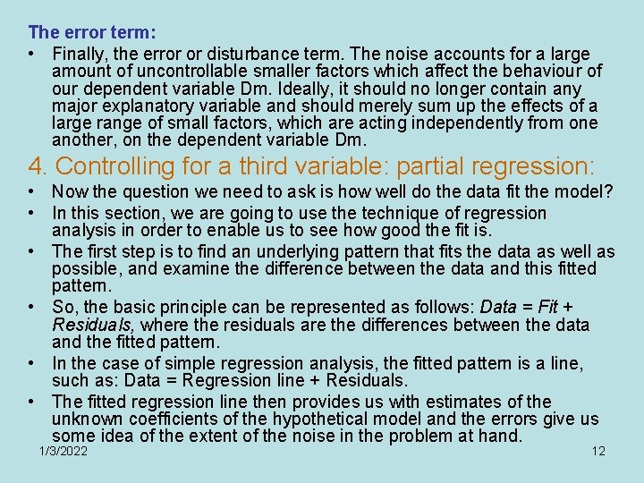
The error term: • Finally, the error or disturbance term. The noise accounts for a large amount of uncontrollable smaller factors which affect the behaviour of our dependent variable Dm. Ideally, it should no longer contain any major explanatory variable and should merely sum up the effects of a large range of small factors, which are acting independently from one another, on the dependent variable Dm. 4. Controlling for a third variable: partial regression: • Now the question we need to ask is how well do the data fit the model? • In this section, we are going to use the technique of regression analysis in order to enable us to see how good the fit is. • The first step is to find an underlying pattern that fits the data as well as possible, and examine the difference between the data and this fitted pattern. • So, the basic principle can be represented as follows: Data = Fit + Residuals, where the residuals are the differences between the data and the fitted pattern. • In the case of simple regression analysis, the fitted pattern is a line, such as: Data = Regression line + Residuals. • The fitted regression line then provides us with estimates of the unknown coefficients of the hypothetical model and the errors give us some idea of the extent of the noise in the problem at hand. 1/3/2022 12

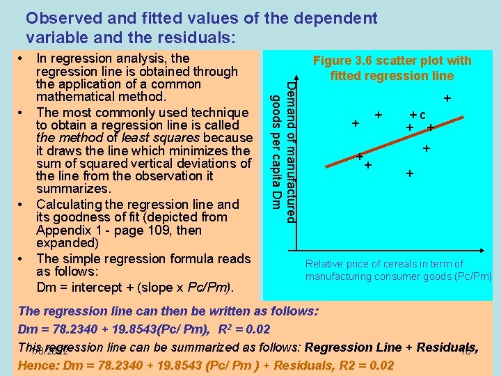
Observed and fitted values of the dependent variable and the residuals: • • • Demand of manufactured goods per capita Dm • In regression analysis, the regression line is obtained through the application of a common mathematical method. The most commonly used technique to obtain a regression line is called the method of least squares because it draws the line which minimizes the sum of squared vertical deviations of the line from the observation it summarizes. Calculating the regression line and its goodness of fit (depicted from Appendix 1 - page 109, then expanded) The simple regression formula reads as follows: Dm = intercept + (slope x Pc/Pm). Figure 3. 6 scatter plot with fitted regression line + + +c + + + Relative price of cereals in term of manufacturing consumer goods (Pc/Pm) The regression line can then be written as follows: Dm = 78. 2340 + 19. 8543(Pc/ Pm), R 2 = 0. 02 This regression line can be summarized as follows: Regression Line + Residuals, 1/3/2022 13 Hence: Dm = 78. 2340 + 19. 8543 (Pc/ Pm ) + Residuals, R 2 = 0. 02

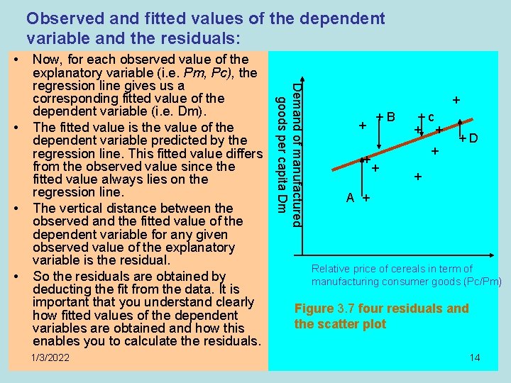
Observed and fitted values of the dependent variable and the residuals: • • • 1/3/2022 Demand of manufactured goods per capita Dm • Now, for each observed value of the explanatory variable (i. e. Pm, Pc), the regression line gives us a corresponding fitted value of the dependent variable (i. e. Dm). The fitted value is the value of the dependent variable predicted by the regression line. This fitted value differs from the observed value since the fitted value always lies on the regression line. The vertical distance between the observed and the fitted value of the dependent variable for any given observed value of the explanatory variable is the residual. So the residuals are obtained by deducting the fit from the data. It is important that you understand clearly how fitted values of the dependent variables are obtained and how this enables you to calculate the residuals. + +B +c + + +D + A + Relative price of cereals in term of manufacturing consumer goods (Pc/Pm) Figure 3. 7 four residuals and the scatter plot 14

• The logical way to solve the Indian example is through using the Multiple Regression, where there are two independent variables: Real Income Y/Pm and relative prices, Pc/Pm, The independent variable is Dm: • The Multiple Regression should be calculated and get this result: • Dm = 37. 2 – 39. 23 Pc/Pm + 0. 17 Y/pm + E • How can we get this result? You should use Excel Tools: • 1. Run excel and enter the data as shown in the example listed below: • Example: • Consumption_Data 1/3/2022 15

Make sure that you understand: • Evaluating economic theory using multiple regression analysis. • Dependent and explanatory variables. • Assumptions of linearity in regression analysis. • Statistical model • Regression model • Method of least squares • Observed and fitted values • Multiplier R 2 and goodness of fit 1/3/2022 16

Consumption_Data 1/3/2022 17