CHAPTER 3 CostVolumeProfit Analysis 2009 Pearson Prentice Hall

- Slides: 19

CHAPTER 3 Cost-Volume-Profit Analysis © 2009 Pearson Prentice Hall. All rights reserved.

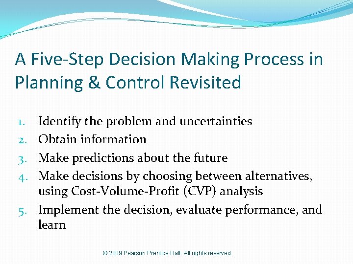
A Five-Step Decision Making Process in Planning & Control Revisited Identify the problem and uncertainties Obtain information Make predictions about the future Make decisions by choosing between alternatives, using Cost-Volume-Profit (CVP) analysis 5. Implement the decision, evaluate performance, and learn 1. 2. 3. 4. © 2009 Pearson Prentice Hall. All rights reserved.

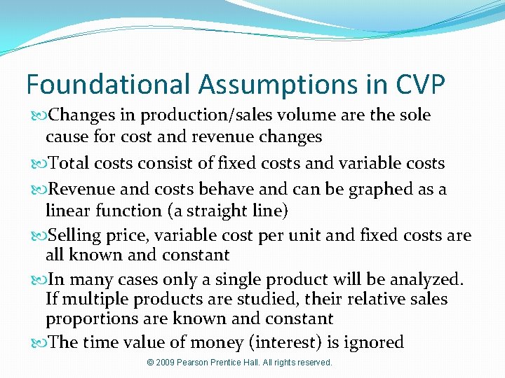
Foundational Assumptions in CVP Changes in production/sales volume are the sole cause for cost and revenue changes Total costs consist of fixed costs and variable costs Revenue and costs behave and can be graphed as a linear function (a straight line) Selling price, variable cost per unit and fixed costs are all known and constant In many cases only a single product will be analyzed. If multiple products are studied, their relative sales proportions are known and constant The time value of money (interest) is ignored © 2009 Pearson Prentice Hall. All rights reserved.

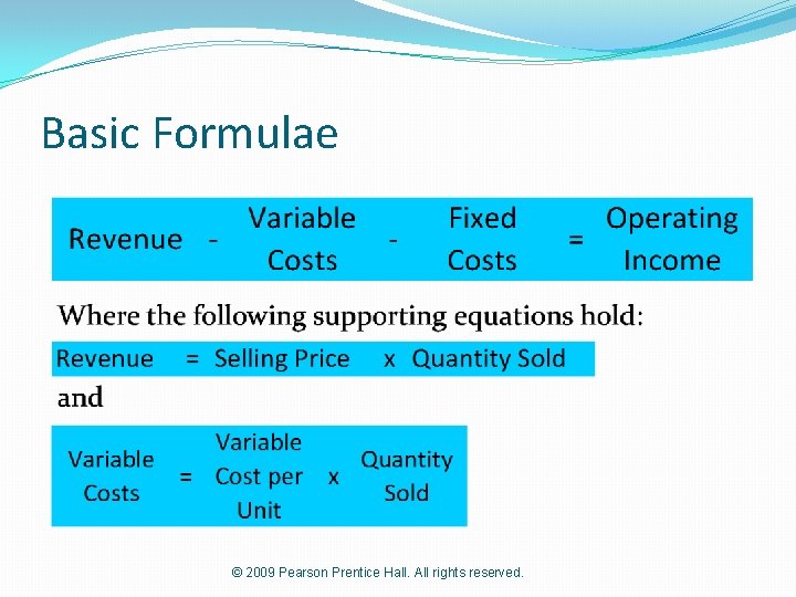
Basic Formulae © 2009 Pearson Prentice Hall. All rights reserved.

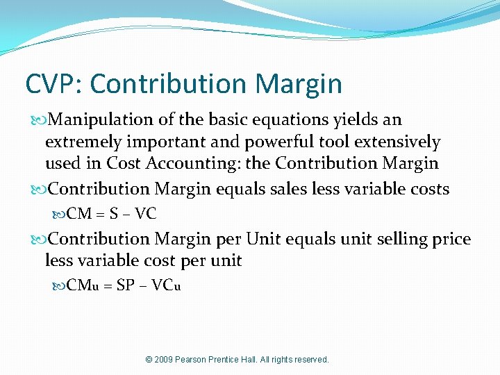
CVP: Contribution Margin Manipulation of the basic equations yields an extremely important and powerful tool extensively used in Cost Accounting: the Contribution Margin equals sales less variable costs CM = S – VC Contribution Margin per Unit equals unit selling price less variable cost per unit CMu = SP – VCu © 2009 Pearson Prentice Hall. All rights reserved.

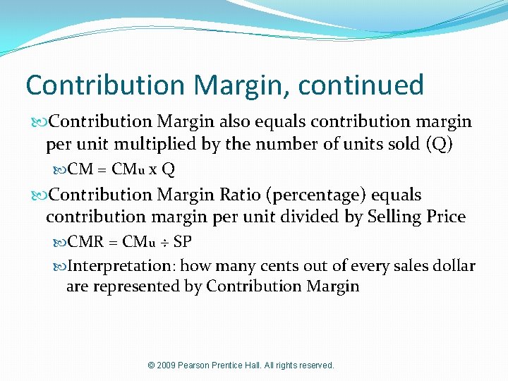
Contribution Margin, continued Contribution Margin also equals contribution margin per unit multiplied by the number of units sold (Q) CM = CMu x Q Contribution Margin Ratio (percentage) equals contribution margin per unit divided by Selling Price CMR = CMu ÷ SP Interpretation: how many cents out of every sales dollar are represented by Contribution Margin © 2009 Pearson Prentice Hall. All rights reserved.

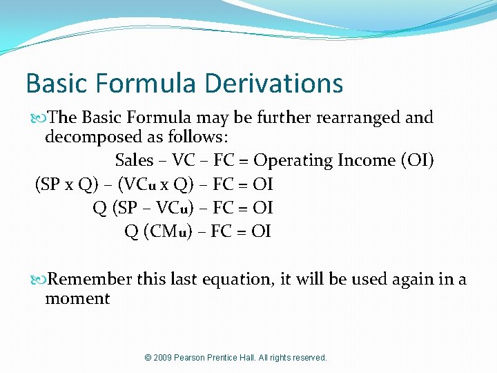
Basic Formula Derivations The Basic Formula may be further rearranged and decomposed as follows: Sales – VC – FC = Operating Income (OI) (SP x Q) – (VCu x Q) – FC = OI Q (SP – VCu) – FC = OI Q (CMu) – FC = OI Remember this last equation, it will be used again in a moment © 2009 Pearson Prentice Hall. All rights reserved.

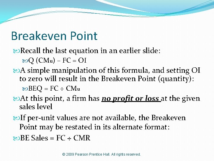
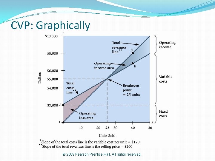
Breakeven Point Recall the last equation in an earlier slide: Q (CMu) – FC = OI A simple manipulation of this formula, and setting OI to zero will result in the Breakeven Point (quantity): BEQ = FC ÷ CMu At this point, a firm has no profit or loss at the given sales level If per-unit values are not available, the Breakeven Point may be restated in its alternate format: BE Sales = FC ÷ CMR © 2009 Pearson Prentice Hall. All rights reserved.

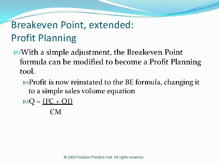
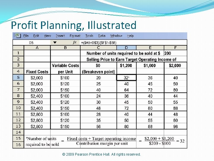
Breakeven Point, extended: Profit Planning With a simple adjustment, the Breakeven Point formula can be modified to become a Profit Planning tool. Profit is now reinstated to the BE formula, changing it to a simple sales volume equation Q = (FC + OI) CM © 2009 Pearson Prentice Hall. All rights reserved.

CVP: Graphically © 2009 Pearson Prentice Hall. All rights reserved.

Profit Planning, Illustrated © 2009 Pearson Prentice Hall. All rights reserved.

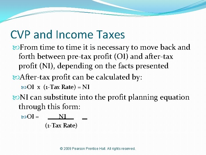
CVP and Income Taxes From time to time it is necessary to move back and forth between pre-tax profit (OI) and after-tax profit (NI), depending on the facts presented After-tax profit can be calculated by: OI x (1 -Tax Rate) = NI can substitute into the profit planning equation through this form: OI = I I NI I (1 -Tax Rate) © 2009 Pearson Prentice Hall. All rights reserved.

Sensitivity Analysis CVP Provides structure to answer a variety of “whatif” scenarios “What” happens to profit “if”: Selling price changes Volume changes Cost structure changes Variable cost per unit changes Fixed cost changes © 2009 Pearson Prentice Hall. All rights reserved.

Margin of Safety One indicator of risk, the Margin of Safety (MOS) measures the distance between budgeted sales and breakeven sales: MOS = Budgeted Sales – BE Sales The MOS Ratio removes the firm’s size from the output, and expresses itself in the form of a percentage: MOS Ratio = MOS ÷ Budgeted Sales © 2009 Pearson Prentice Hall. All rights reserved.

Operating Leverage (OL) is the effect that fixed costs have on changes in operating income as changes occur in units sold, expressed as changes in contribution margin OL = Contribution Margin Operating Income Notice these two items are identical, except for fixed costs © 2009 Pearson Prentice Hall. All rights reserved.

Effects of Sales-Mix on CVP The formulae presented to this point have assumed a single product is produced and sold A more realistic scenario involves multiple products sold, in different volumes, with different costs The same formulae are used, but instead use average contribution margins for bundles of products. © 2009 Pearson Prentice Hall. All rights reserved.

Multiple Cost Drivers Variable costs may arise from multiple cost drivers or activities. A separate variable cost needs to be calculated for each driver. Examples include: Customer or patient count Passenger miles Patient days Student credit-hours © 2009 Pearson Prentice Hall. All rights reserved.

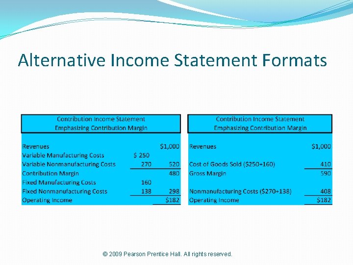
Alternative Income Statement Formats © 2009 Pearson Prentice Hall. All rights reserved.

© 2009 Pearson Prentice Hall. All rights reserved.