Chapter 3 By Miss Mardianaliza Othman 1 2

Chapter 3 By: Miss Mardianaliza Othman 1

2 Chapter Objectives Upon the learning the material presented in this chapter, you should be able to : 1. Calculate the magnetic force and torque on a current carrying wire. 2. Apply the Biot-Savart’s law 3. Aplply the Ampere’s law 4. Calculate the inductance of a solenoid, a coaxial transmission and other configurations 5. Evaluate the magnetic energy

3 Chapter Outlines ü Magnetic forces and torques ü The Biot-Savart law ü Magnetic force between two parallel conductors ü Maxwell’s magnetostatic Equations ü Vector magnetic potential ü Magnetic properties of materials ü Magnetic Boundary Conditions ü Inductances ü Magnetic Energy

INTRODUCTION Magnetism and electricity were considered distinct phenomena until 1820 when Hans Christian Oersted introduced an experiment that showed a compass needle deflecting when in proximity to current carrying wire. He used compass to show that current produces magnetic fields that loop around the conductor. The field grows weaker as it moves away from the source of current. 4

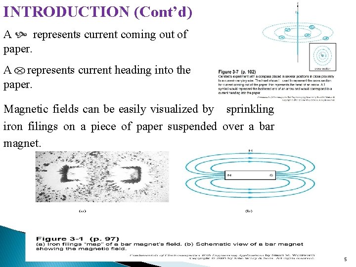
INTRODUCTION (Cont’d) A represents current coming out of paper. A represents current heading into the paper. Magnetic fields can be easily visualized by sprinkling iron filings on a piece of paper suspended over a bar magnet. 5

INTRODUCTION (Cont’d) The principle of magnetism is widely used in many applications: Ø Motors and generators Ø Magnetic memory Ø Microphones and speakers Ø Magnetically levitated high-speed vehicle. The field lines are in terms of the magnetic field intensity, H in units of amps per meter. This is analogous to the volts per meter units for electric field intensity, E. Magnetic field will be introduced in a manner paralleling our treatment to electric fields. 6

Maxwell’s equations for magnetostatic: where J is the current density The magnetic flux density B and the magnetic field intensity H are related by where μ is medium magnetic permeability μo = free space permeability = 4π 10 -7 H/m μr = relative permeability of medium 7

3 -1 MAGNETIC FORCES AND TORQUES § The electric field E at a point in space is defined as the electric force Fe per unit charge acting on a test charge when placed at that point. or § Fe = q E (N) When charged particle moving with a velocity u, magnetic force Fm is produced. Fm = q u x B (N) where B = magnetic flux density (N/C-m/s or Tesla T) § When charged particle has E and B, total electromagnetic force is This force is known as Lorentz force 8

Exercise 3. 1 The point charge Q = 18 n. C has a velocity of 5 x 10 -6 m/s in the direction av = 0. 60 ax + 0. 75 ay + 0. 30 az. Calculate the magnitude of force exerted on the charge by the field : a) B = - 3 ax + 4 ay + 6 az m. T; 660 μN b) E = - 3 ax + 4 ay + 6 az k. V/m 140 μN c) B and E acting together. 670 μN 9

Magnetic Force on a Current-Carrying Conductor To find a force on a current element, consider a line conducting current in the presence of magnetic field with differential segment d. Q of charge moving with velocity u: But, so Since d. Q/dt corresponds to the current I in the line, We can find the force from a collection of current elements 10

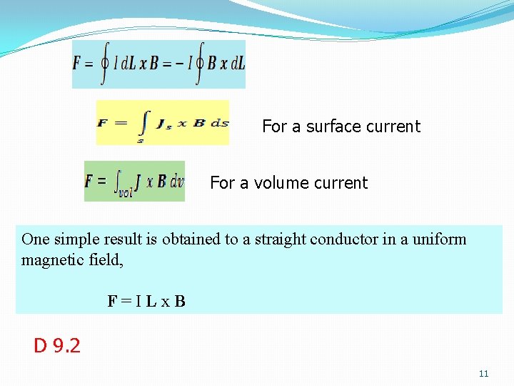
For a surface current For a volume current One simple result is obtained to a straight conductor in a uniform magnetic field, F=ILx. B D 9. 2 11

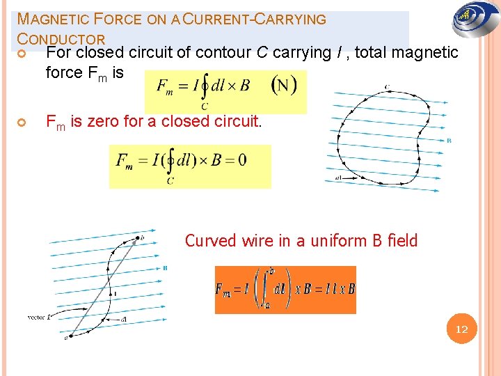
MAGNETIC FORCE ON A CURRENT-CARRYING CONDUCTOR For closed circuit of contour C carrying I , total magnetic force Fm is zero for a closed circuit. Curved wire in a uniform B field 12

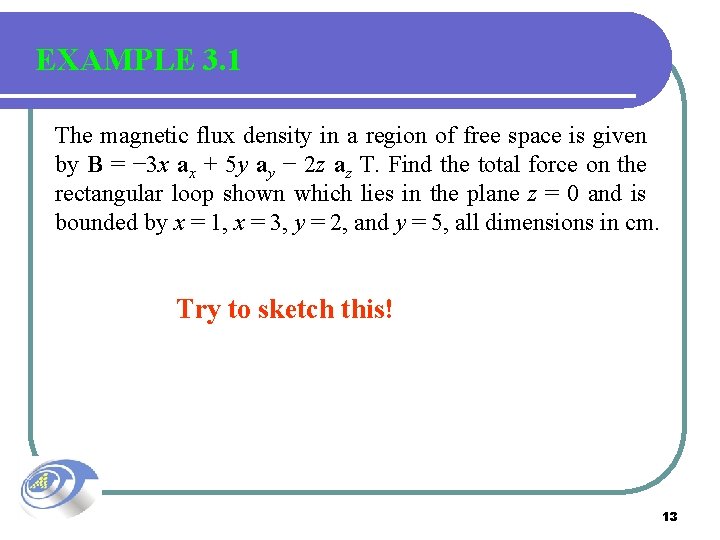
EXAMPLE 3. 1 The magnetic flux density in a region of free space is given by B = − 3 x ax + 5 y ay − 2 z az T. Find the total force on the rectangular loop shown which lies in the plane z = 0 and is bounded by x = 1, x = 3, y = 2, and y = 5, all dimensions in cm. Try to sketch this! 13

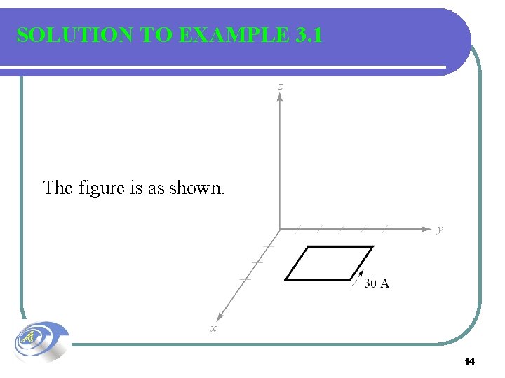
SOLUTION TO EXAMPLE 3. 1 The figure is as shown. 14

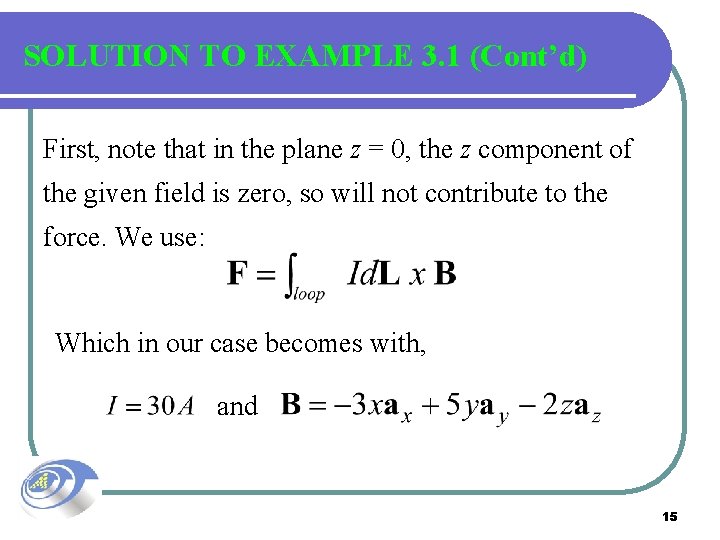
SOLUTION TO EXAMPLE 3. 1 (Cont’d) First, note that in the plane z = 0, the z component of the given field is zero, so will not contribute to the force. We use: Which in our case becomes with, and 15

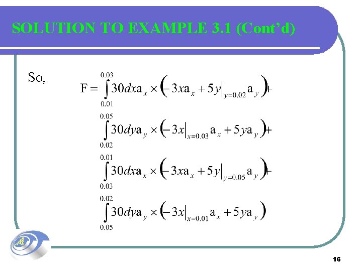
SOLUTION TO EXAMPLE 3. 1 (Cont’d) So, 16

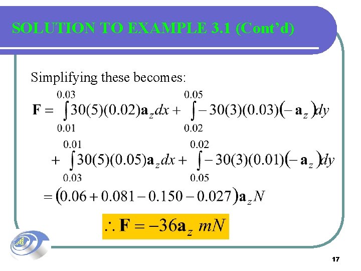
SOLUTION TO EXAMPLE 3. 1 (Cont’d) Simplifying these becomes: 17

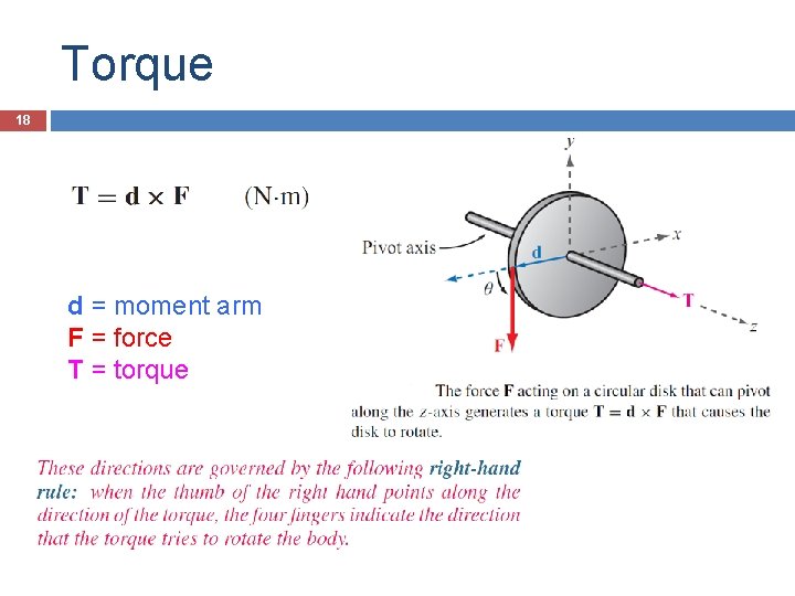
Torque 18 d = moment arm F = force T = torque

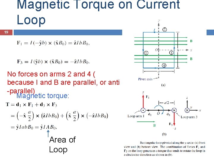
Magnetic Torque on Current Loop 19 No forces on arms 2 and 4 ( because I and B are parallel, or anti -parallel) Magnetic torque: Area of Loop

Inclined Loop 20 For a loop with N turns and whose surface normal is at angle theta relative to B direction:

21

3 -2 Biot-Savart’s Law State: At any point P, the magnitude of the magnetic field intensity produced by the differential element is proportional to the product of the current, the magnitude of the differential length, and the sine of the angle lying between the filament and a line connecting the filament to the point P at which the field is desired; also the magnitude of the magnetic field intensity is inversely proportional to the square of the distance from the differential element to the point P. 22

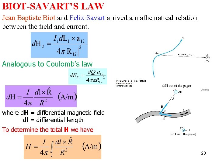
BIOT-SAVART’S LAW Jean Baptiste Biot and Felix Savart arrived a mathematical relation between the field and current. Analogous to Coulomb’s law where d. H = differential magnetic field dl = differential length To determine the total H we have 23

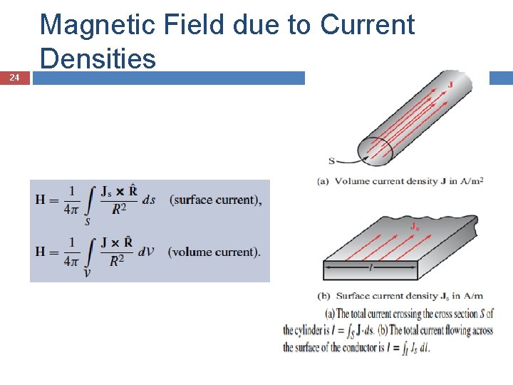
24 Magnetic Field due to Current Densities

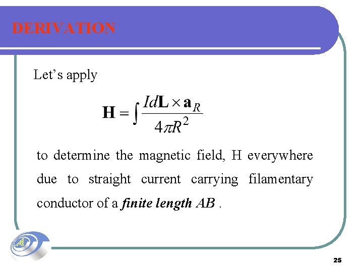
DERIVATION Let’s apply to determine the magnetic field, H everywhere due to straight current carrying filamentary conductor of a finite length AB. 25

DERIVATION (Cont’d) 26

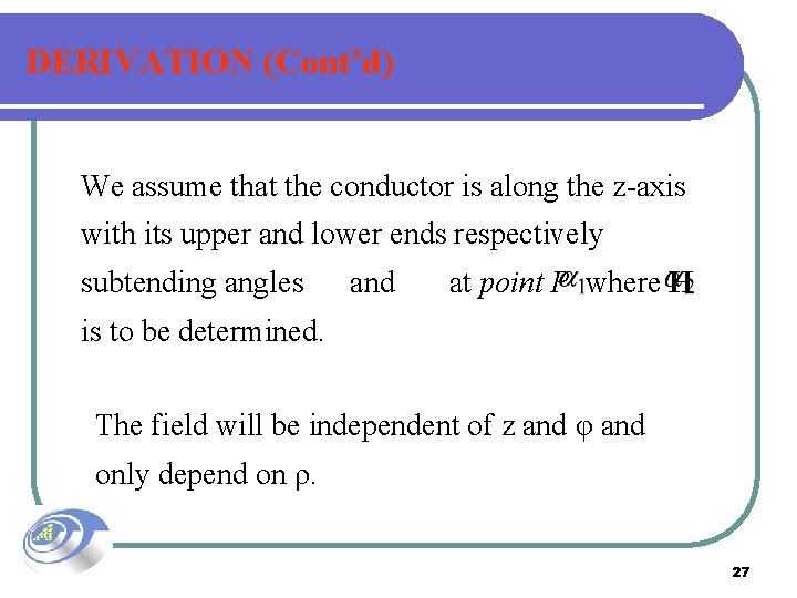
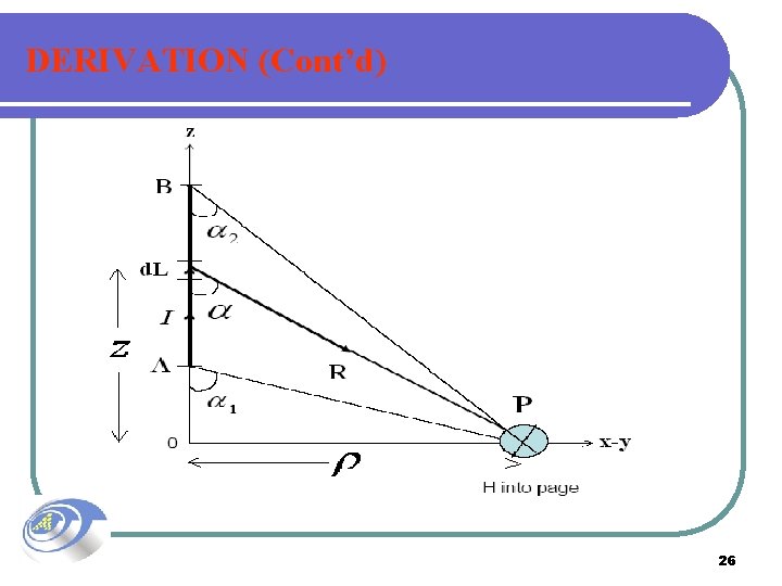
DERIVATION (Cont’d) We assume that the conductor is along the z-axis with its upper and lower ends respectively subtending angles and at point P where H is to be determined. The field will be independent of z and φ and only depend on ρ. 27

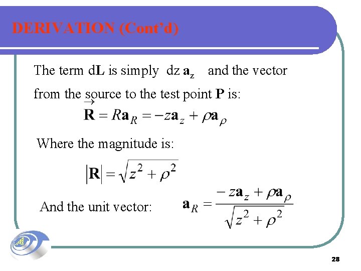
DERIVATION (Cont’d) The term d. L is simply dz az and the vector from the source to the test point P is: Where the magnitude is: And the unit vector: 28

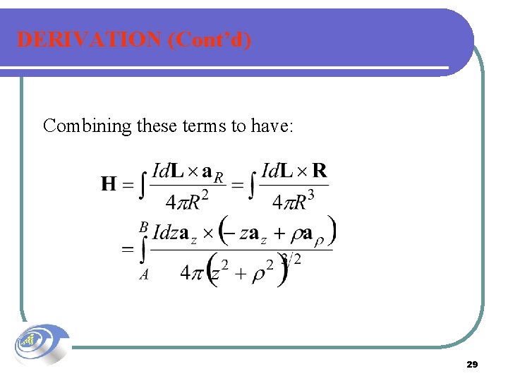
DERIVATION (Cont’d) Combining these terms to have: 29

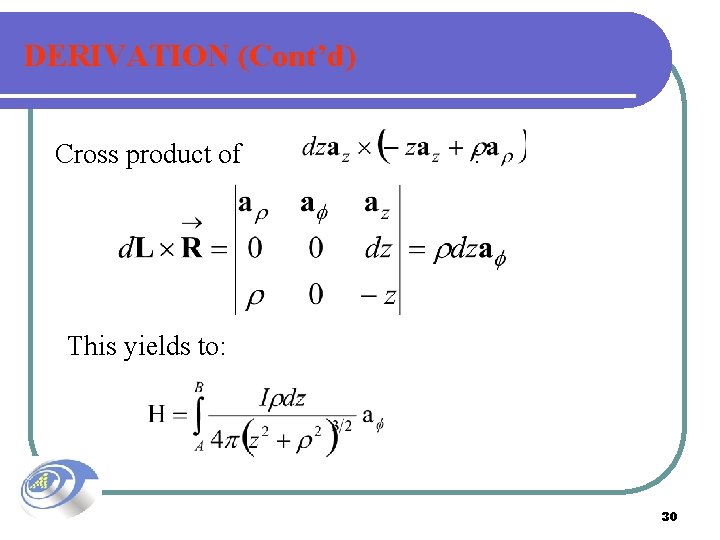
DERIVATION (Cont’d) Cross product of : This yields to: 30

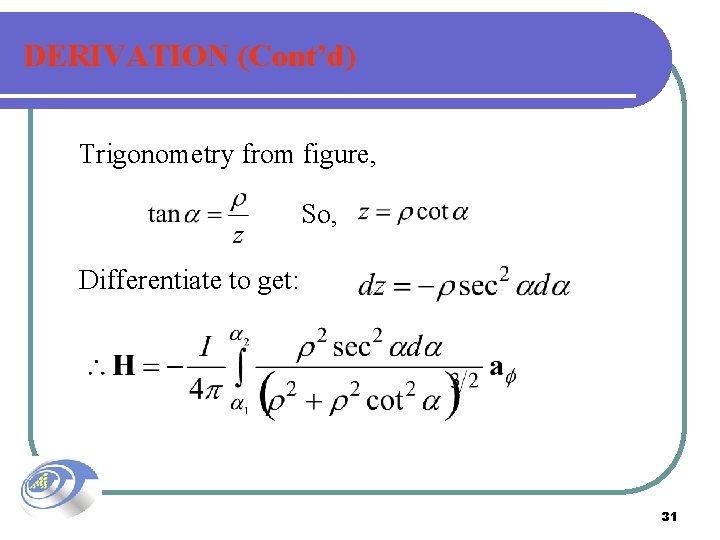
DERIVATION (Cont’d) Trigonometry from figure, So, Differentiate to get: 31

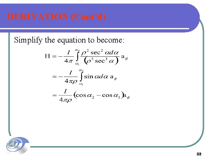
DERIVATION (Cont’d) Simplify the equation to become: 32

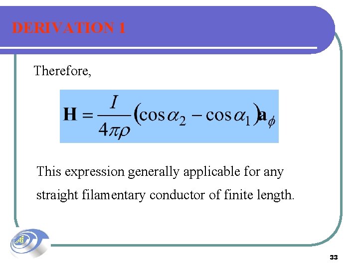
DERIVATION 1 Therefore, This expression generally applicable for any straight filamentary conductor of finite length. 33

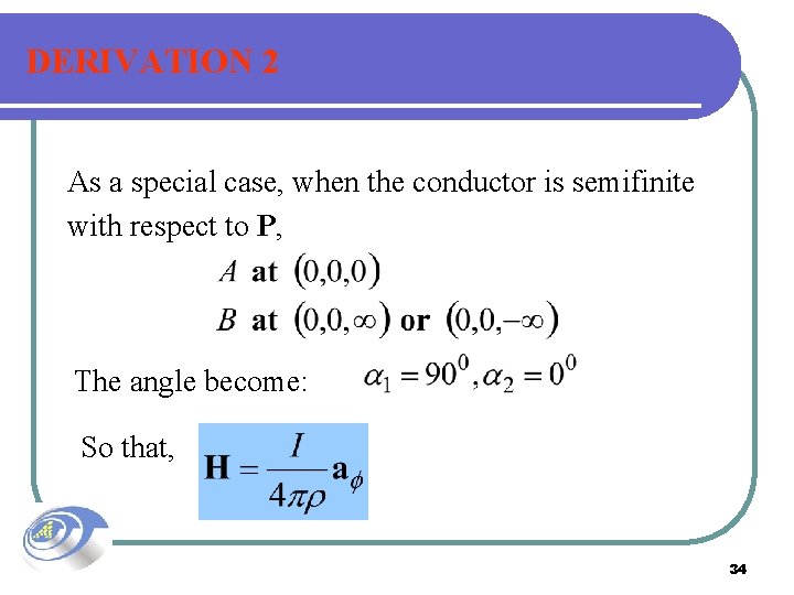
DERIVATION 2 As a special case, when the conductor is semifinite with respect to P, The angle become: So that, 34

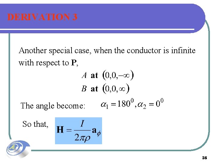
DERIVATION 3 Another special case, when the conductor is infinite with respect to P, The angle become: So that, 35

36

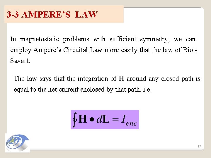
3 -3 AMPERE’S LAW In magnetostatic problems with sufficient symmetry, we can employ Ampere’s Circuital Law more easily that the law of Biot. Savart. The law says that the integration of H around any closed path is equal to the net current enclosed by that path. i. e. 37

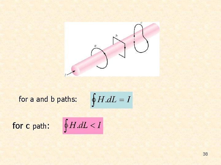
for a and b paths: for c path: 38

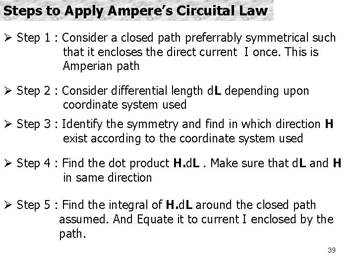
Steps to Apply Ampere’s Circuital Law Ø Step 1 : Consider a closed path preferrably symmetrical such that it encloses the direct current I once. This is Amperian path Ø Step 2 : Consider differential length d. L depending upon coordinate system used Ø Step 3 : Identify the symmetry and find in which direction H exist according to the coordinate system used Ø Step 4 : Find the dot product H. d. L. Make sure that d. L and H in same direction Ø Step 5 : Find the integral of H. d. L around the closed path assumed. And Equate it to current I enclosed by the path. 39

AMPERE’S LAW (Cont’d) • The line integral of H around the path is termed the circulation of H. • To solve for H in given symmetrical current distribution, it is important to make a careful selection of an Amperian Path (analogous to gaussian surface) that is everywhere either tangential or normal to H. • The direction of the circulation is chosen such that the right hand rule is satisfied. 40

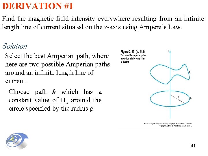
DERIVATION #1 Find the magnetic field intensity everywhere resulting from an infinite length line of current situated on the z-axis using Ampere’s Law. Solution Select the best Amperian path, where are two possible Amperian paths around an infinite length line of current. Choose path b which has a constant value of Hφ around the circle specified by the radius ρ 41

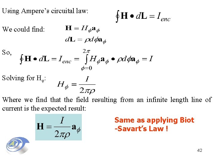
Using Ampere’s circuital law: We could find: So, Solving for Hφ: Where we find that the field resulting from an infinite length line of current is the expected result: Same as applying Biot -Savart’s Law ! 42

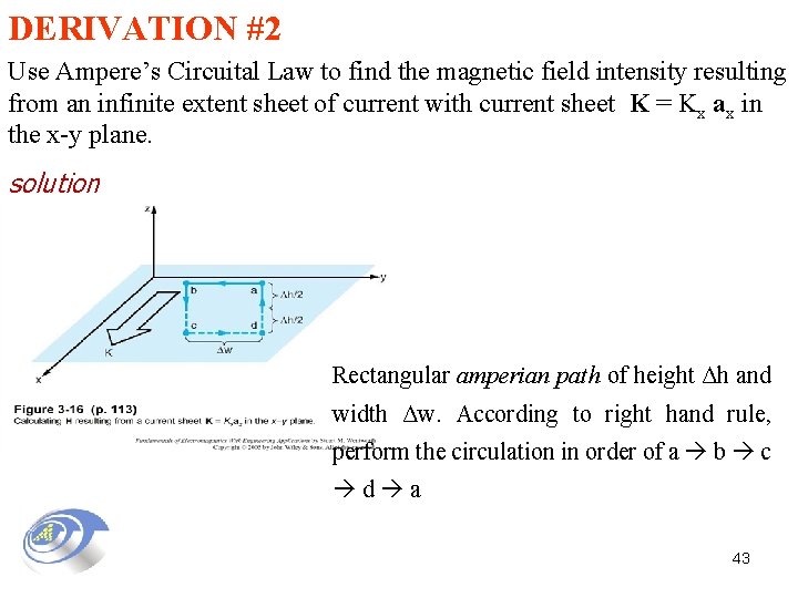
DERIVATION #2 Use Ampere’s Circuital Law to find the magnetic field intensity resulting from an infinite extent sheet of current with current sheet K = Kx ax in the x-y plane. solution Rectangular amperian path of height Δh and width Δw. According to right hand rule, perform the circulation in order of a b c d a 43

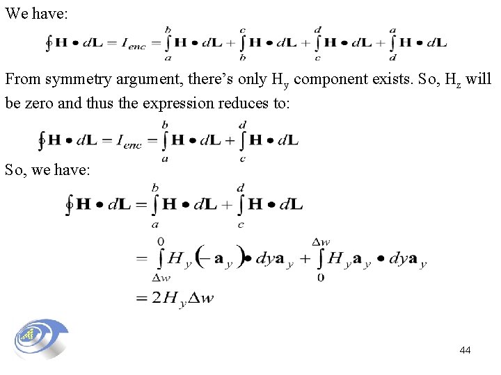
We have: From symmetry argument, there’s only Hy component exists. So, Hz will be zero and thus the expression reduces to: So, we have: 44

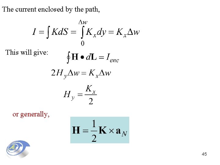
The current enclosed by the path, This will give: or generally, 45

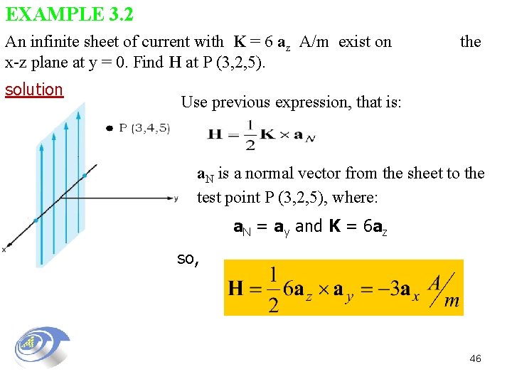
EXAMPLE 3. 2 An infinite sheet of current with K = 6 az A/m exist on x-z plane at y = 0. Find H at P (3, 2, 5). solution the Use previous expression, that is: a. N is a normal vector from the sheet to the test point P (3, 2, 5), where: a. N = ay and K = 6 az so, 46

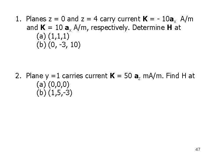
1. Planes z = 0 and z = 4 carry current K = - 10 ax A/m and K = 10 ax A/m, respectively. Determine H at (a) (1, 1, 1) (b) (0, -3, 10) 2. Plane y =1 carries current K = 50 az m. A/m. Find H at (a) (0, 0, 0) (b) (1, 5, -3) 47

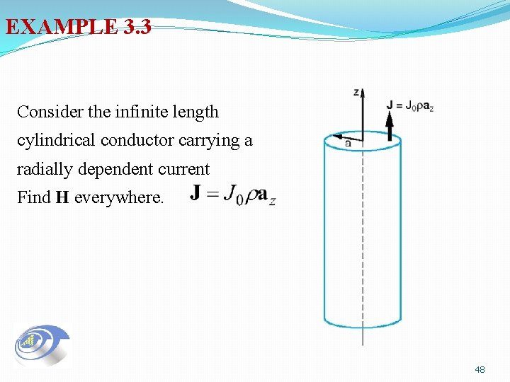
EXAMPLE 3. 3 Consider the infinite length cylindrical conductor carrying a radially dependent current Find H everywhere. 48

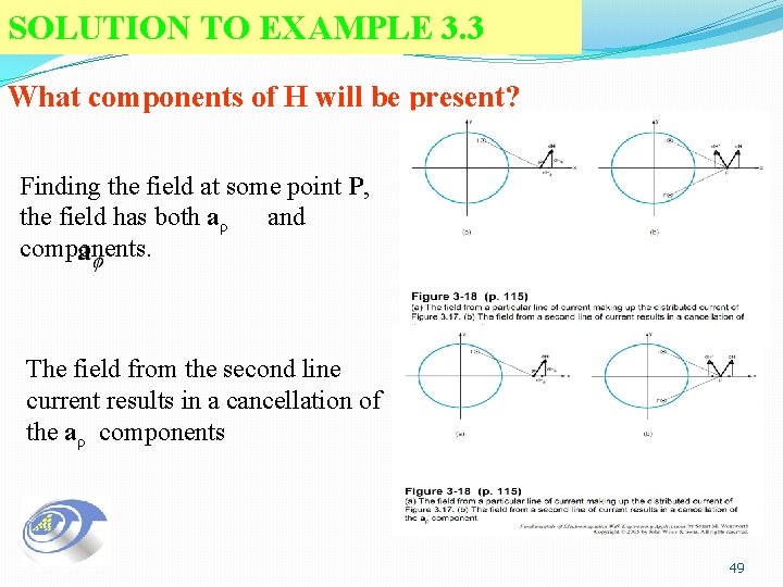
SOLUTION TO EXAMPLE 3. 3 What components of H will be present? Finding the field at some point P, the field has both aρ and components. The field from the second line current results in a cancellation of the aρ components 49

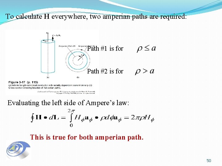
To calculate H everywhere, two amperian paths are required: Path #1 is for Path #2 is for Evaluating the left side of Ampere’s law: This is true for both amperian path. 50

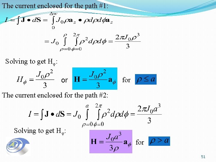
The current enclosed for the path #1: Solving to get Hφ: or for The current enclosed for the path #2: Solving to get Hφ: for 51

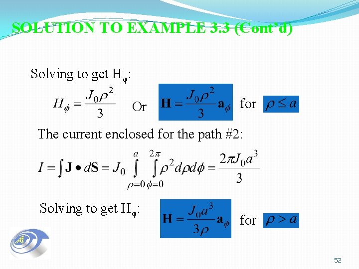
SOLUTION TO EXAMPLE 3. 3 (Cont’d) Solving to get Hφ: Or for The current enclosed for the path #2: Solving to get Hφ: for 52

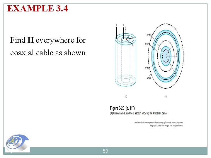
EXAMPLE 3. 4 Find H everywhere for coaxial cable as shown. Syaf Hasan 53

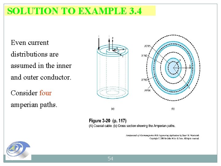
SOLUTION TO EXAMPLE 3. 4 Even current distributions are assumed in the inner and outer conductor. Consider four amperian paths. Syaf Hasan 54

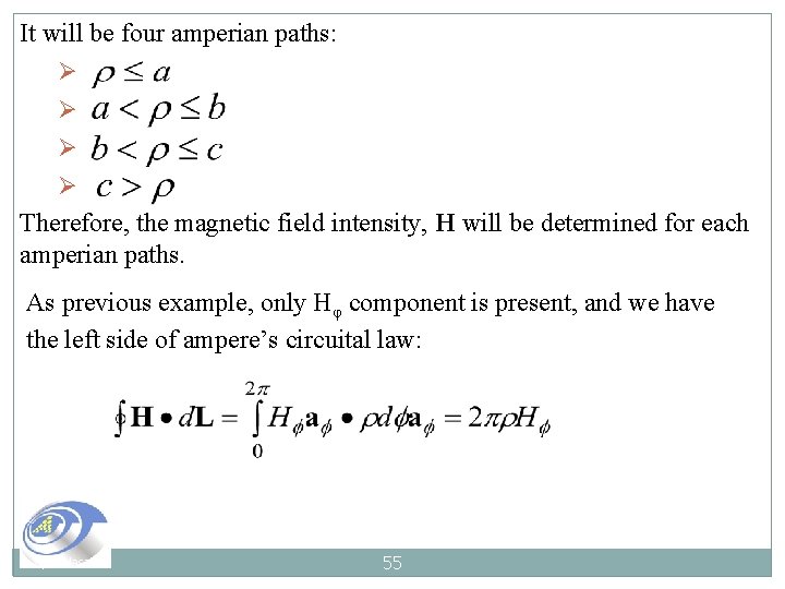
It will be four amperian paths: Ø Ø Therefore, the magnetic field intensity, H will be determined for each amperian paths. As previous example, only Hφ component is present, and we have the left side of ampere’s circuital law: Syaf Hasan 55

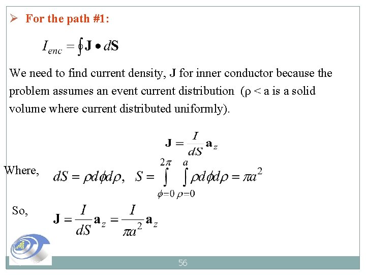
Ø For the path #1: We need to find current density, J for inner conductor because the problem assumes an event current distribution (ρ < a is a solid volume where current distributed uniformly). Where, So, Syaf Hasan 56

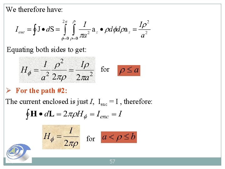
We therefore have: Equating both sides to get: for Ø For the path #2: The current enclosed is just I, Ienc = I , therefore: for Syaf Hasan 57

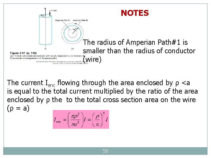
NOTES The radius of Amperian Path#1 is smaller than the radius of conductor (wire) The current Ienc flowing through the area enclosed by ρ <a is equal to the total current multiplied by the ratio of the area enclosed by ρ the total cross section area on the wire (ρ = a) 58

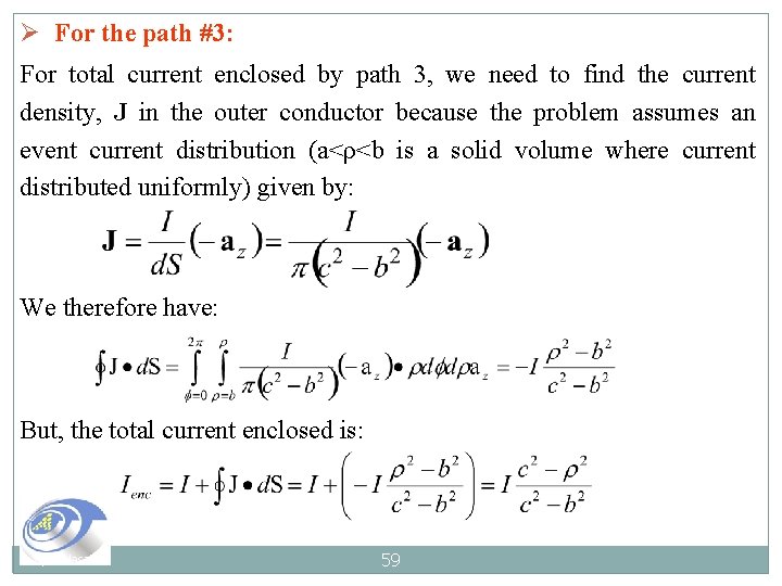
Ø For the path #3: For total current enclosed by path 3, we need to find the current density, J in the outer conductor because the problem assumes an event current distribution (a<ρ<b is a solid volume where current distributed uniformly) given by: We therefore have: But, the total current enclosed is: Syaf Hasan 59

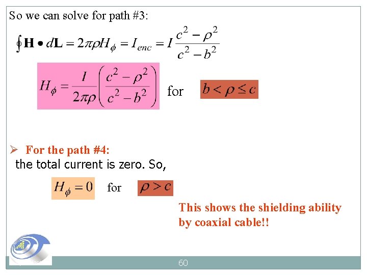
So we can solve for path #3: for Ø For the path #4: the total current is zero. So, for This shows the shielding ability by coaxial cable!! Syaf Hasan 60

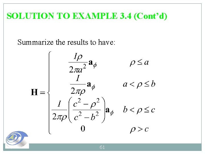
SOLUTION TO EXAMPLE 3. 4 (Cont’d) Summarize the results to have: Syaf Hasan 61

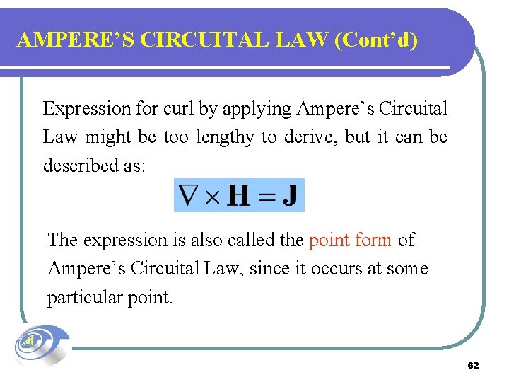
AMPERE’S CIRCUITAL LAW (Cont’d) Expression for curl by applying Ampere’s Circuital Law might be too lengthy to derive, but it can be described as: The expression is also called the point form of Ampere’s Circuital Law, since it occurs at some particular point. 62

Find J at (2 m, 1 m, 3 m) if H = 2 xy 2 az A/m. 63

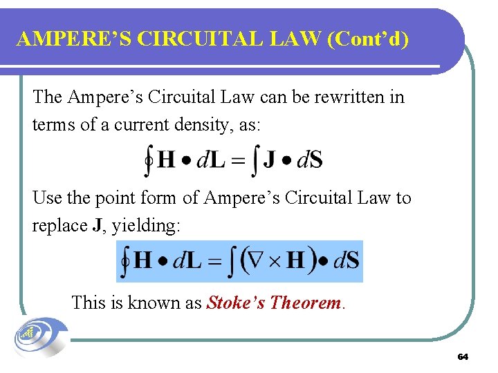
AMPERE’S CIRCUITAL LAW (Cont’d) The Ampere’s Circuital Law can be rewritten in terms of a current density, as: Use the point form of Ampere’s Circuital Law to replace J, yielding: This is known as Stoke’s Theorem. 64

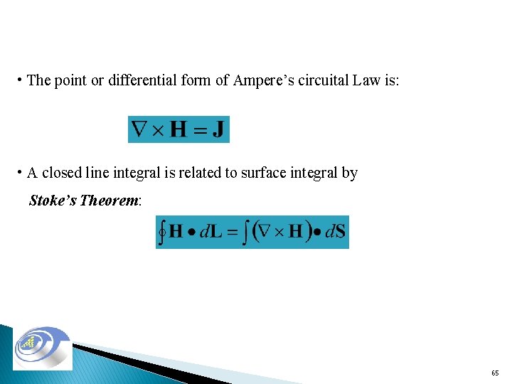
• The point or differential form of Ampere’s circuital Law is: • A closed line integral is related to surface integral by Stoke’s Theorem: 65

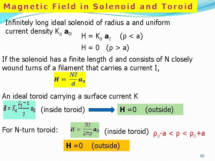
Magnetic Field in Solenoid and Toroid Infinitely long ideal solenoid of radius a and uniform current density Ka aΦ H = Ka az (ρ < a) H = 0 (ρ > a) If the solenoid has a finite length d and consists of N closely wound turns of a filament that carries a current I, An ideal toroid carrying a surface current K (inside toroid) For N-turn toroid: H =0 (outside) (inside toroid) ρo-a < ρo+a H =0 (outside) 66

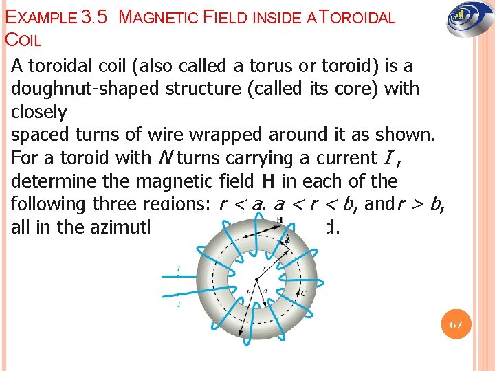
EXAMPLE 3. 5 MAGNETIC FIELD INSIDE A TOROIDAL COIL A toroidal coil (also called a torus or toroid) is a doughnut-shaped structure (called its core) with closely spaced turns of wire wrapped around it as shown. For a toroid with N turns carrying a current I , determine the magnetic field H in each of the following three regions: r < a, a < r < b, andr > b, all in the azimuthal plane of the toroid. 67

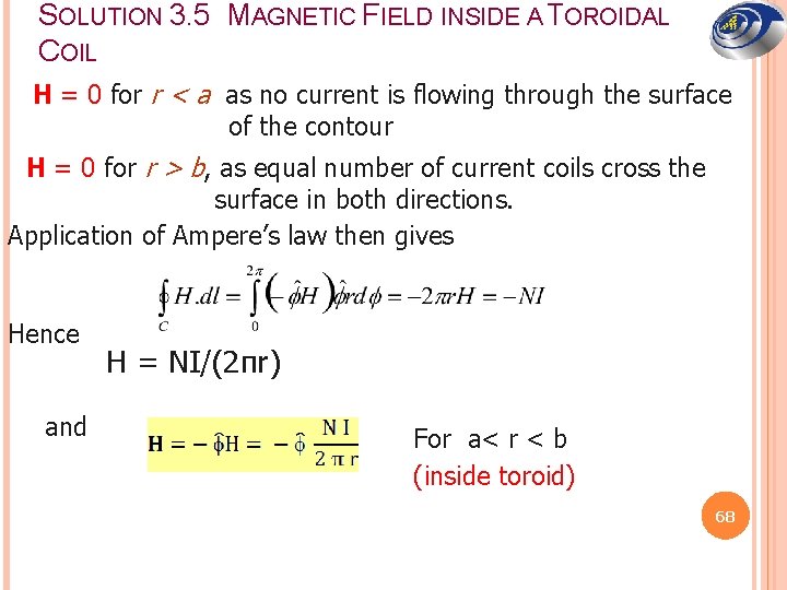
SOLUTION 3. 5 MAGNETIC FIELD INSIDE A TOROIDAL COIL H = 0 for r < a as no current is flowing through the surface of the contour H = 0 for r > b, as equal number of current coils cross the surface in both directions. Application of Ampere’s law then gives Hence and H = NI/(2πr) For a< r < b (inside toroid) 68

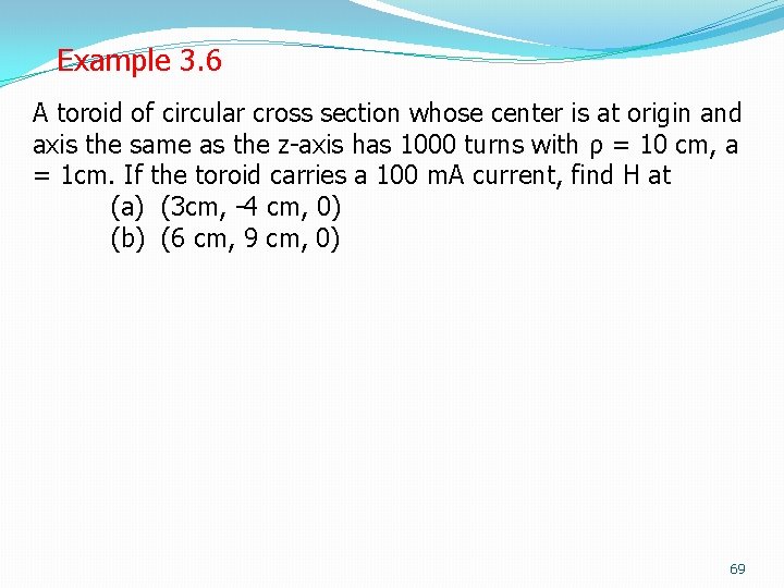
Example 3. 6 A toroid of circular cross section whose center is at origin and axis the same as the z-axis has 1000 turns with ρ = 10 cm, a = 1 cm. If the toroid carries a 100 m. A current, find H at (a) (3 cm, -4 cm, 0) (b) (6 cm, 9 cm, 0) 69

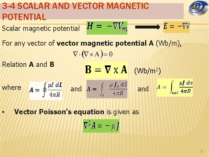
3 -4 SCALAR AND VECTOR MAGNETIC POTENTIAL Syaf Hasan Scalar magnetic potential For any vector of vector magnetic potential A (Wb/m), Relation A and B where • (Wb/m 2) and Vector Poisson’s equation is given as 70

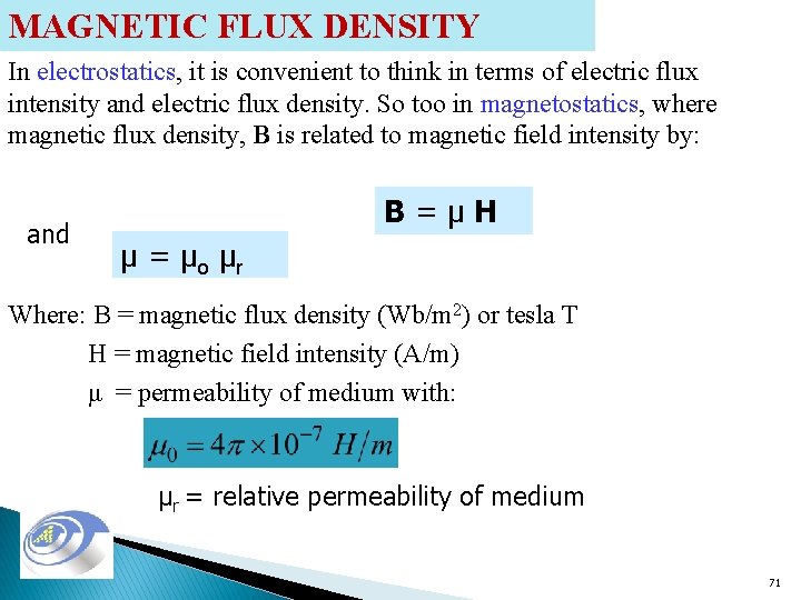
MAGNETIC FLUX DENSITY In electrostatics, it is convenient to think in terms of electric flux intensity and electric flux density. So too in magnetostatics, where magnetic flux density, B is related to magnetic field intensity by: and B=μH μ = μo μr Where: B = magnetic flux density (Wb/m 2) or tesla T H = magnetic field intensity (A/m) μ = permeability of medium with: μr = relative permeability of medium 71

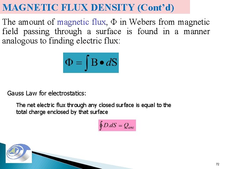
MAGNETIC FLUX DENSITY (Cont’d) The amount of magnetic flux, Φ in Webers from magnetic field passing through a surface is found in a manner analogous to finding electric flux: Gauss Law for electrostatics: The net electric flux through any closed surface is equal to the total charge enclosed by that surface 72

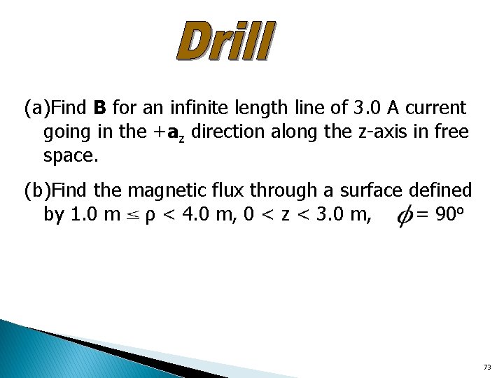
(a)Find B for an infinite length line of 3. 0 A current going in the +az direction along the z-axis in free space. (b)Find the magnetic flux through a surface defined by 1. 0 m ρ < 4. 0 m, 0 < z < 3. 0 m, = 90 o 73

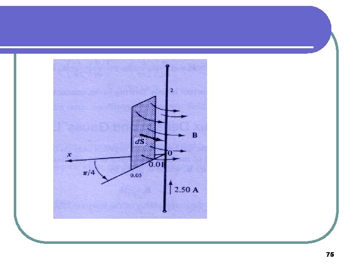
EXAMPLE 3. 7 Find the flux crossing the portion of the plane φ = π/4 defined by 0. 01 m < r < 0. 05 m and 0 < z < 2 m in free space. A current filament of 2. 5 A is along the z axis in the az direction. Try to sketch this! 74

75

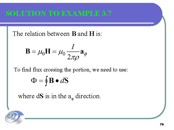
SOLUTION TO EXAMPLE 3. 7 The relation between B and H is: To find flux crossing the portion, we need to use: where d. S is in the aφ direction. 76

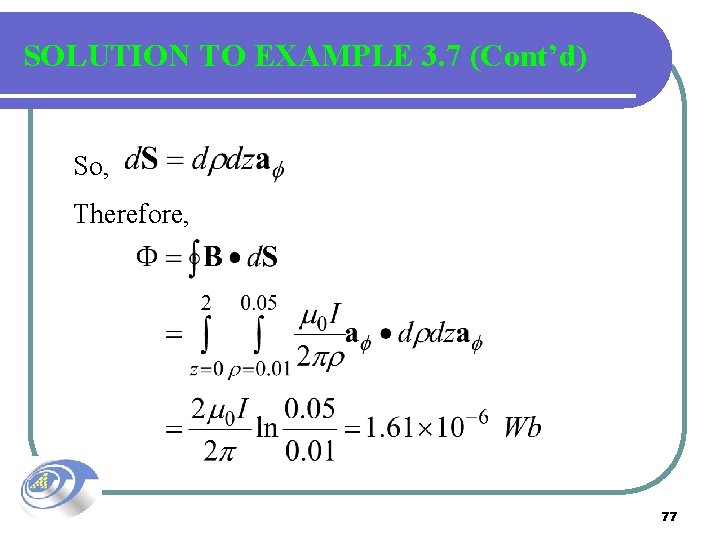
SOLUTION TO EXAMPLE 3. 7 (Cont’d) So, Therefore, 77

3 -5 MAGNETIC PROPERTIES OF MATERIALS Syaf Hasan � � Magnetic behavior is due to the interaction of dipole and field. 6 types of magnetic materials: Ø Ø Ø Diamagnetic, Paramagnetic, Ferromagnetic. Antiferromagnetic Ferrimagnetic Superparamagnetic 78

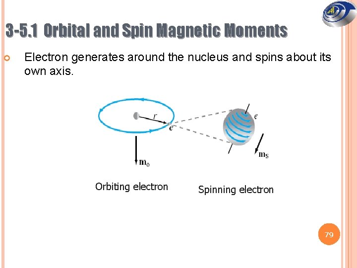
3 -5. 1 Orbital and Spin Magnetic Moments Electron generates around the nucleus and spins about its own axis. Orbiting electron Spinning electron 79

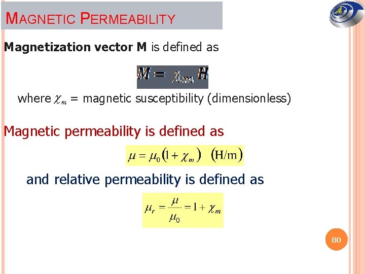
MAGNETIC PERMEABILITY Magnetization vector M is defined as where = magnetic susceptibility (dimensionless) Magnetic permeability is defined as and relative permeability is defined as 80

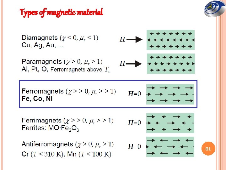
Types of magnetic material 81

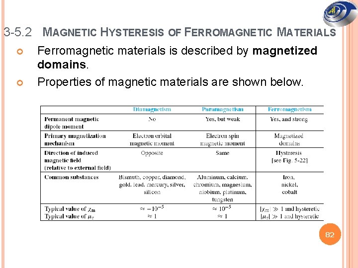
3 -5. 2 MAGNETIC HYSTERESIS OF FERROMAGNETIC MATERIALS Ferromagnetic materials is described by magnetized domains. Properties of magnetic materials are shown below. 82

Diamagnetic materials create a magnetic field in opposition to an externally applied magnetic field. It is a quantum mechanical effect that occurs in all materials. Paramagnetism is a form of magnetism whereby certain materials are attracted by an externally applied magnetic field. Ferromagnetism is the physical theory which explains how materials become magnets. Syaf Hasan 83

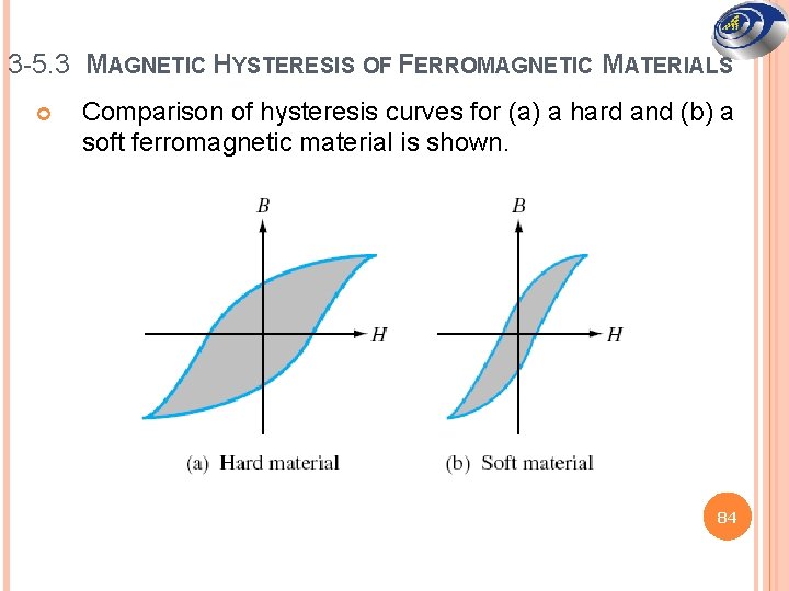
3 -5. 3 MAGNETIC HYSTERESIS OF FERROMAGNETIC MATERIALS Comparison of hysteresis curves for (a) a hard and (b) a soft ferromagnetic material is shown. 84

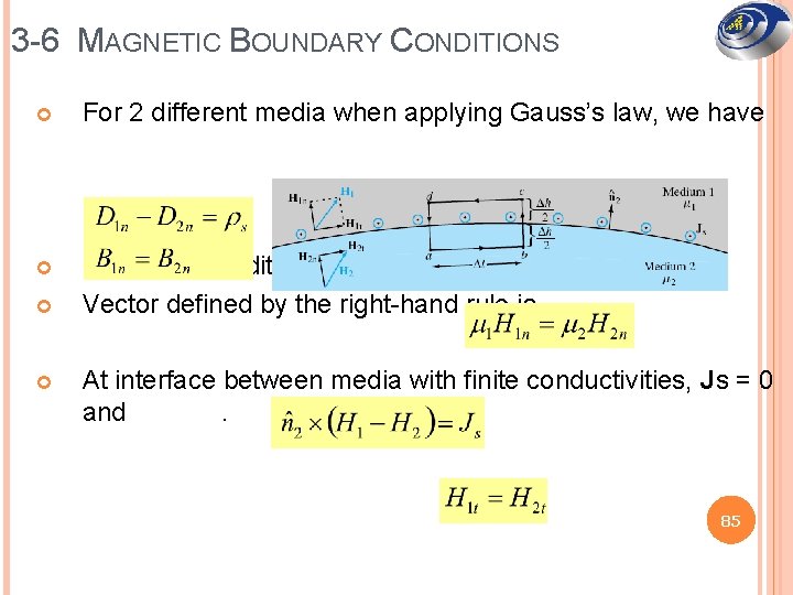
3 -6 MAGNETIC BOUNDARY CONDITIONS For 2 different media when applying Gauss’s law, we have Boundary condition for H is. Vector defined by the right-hand rule is At interface between media with finite conductivities, Js = 0 and. 85

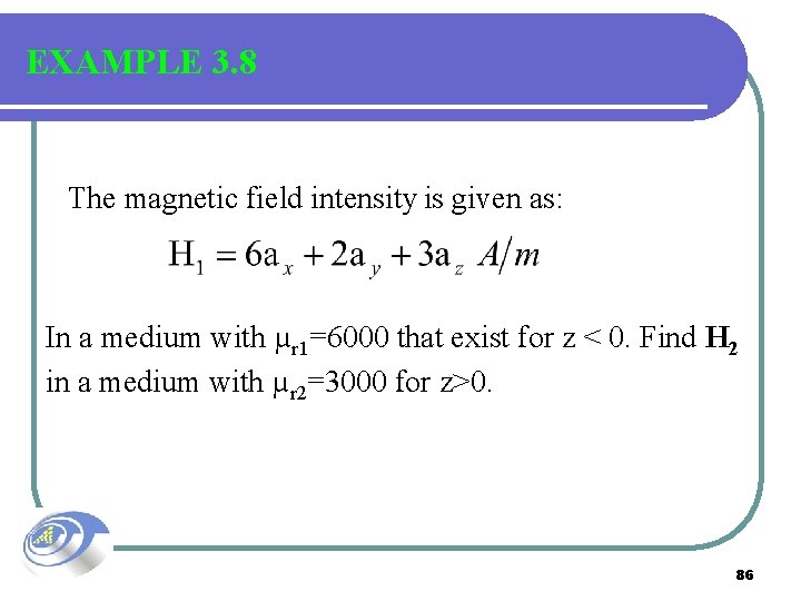
EXAMPLE 3. 8 The magnetic field intensity is given as: In a medium with µr 1=6000 that exist for z < 0. Find H 2 in a medium with µr 2=3000 for z>0. 86

First to break H 1 into normal component (step 1) and tangential component (step 2). With no current at the interface, the tangential component is the same as both sides of the boundary (step 3). Next we find Bn 1 by multiplying Hn 1 by the permeability in medium 1 (step 4). This normal component B is the same on both sides of the boundary (step 5), and then we can find Hn 2 by dividing Bn 2 by the permeability of medium 2 (step 6). The last step is to sum the fields (step 7). 87

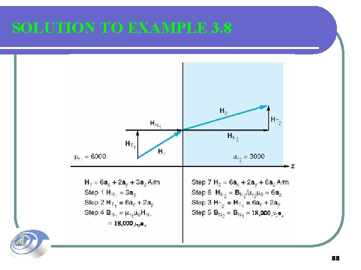
SOLUTION TO EXAMPLE 3. 8 88