Chapter 3 b Continuous RVs Expected Value Joint

Chapter 3 b Continuous RVs Expected Value Joint Densities MGFs Poisson and Normal Distributions
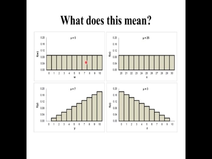
 about")
Unusual Events Unusual Event Principle: If we make an assumption (or a claim) about a random experiment, and then observe an event with a very small probability based on that assumption (called an “unusual event”), then we conclude that the assumption is most likely incorrect.
 and represents the number")
Unusual Events Unusual Event Guideline: If X is b(n, p) and represents the number of successes in a random experiment, then an observed event consisting of exactly x successes is considered “unusual” if

Example 2. 3. 7 Suppose a university student body consists of 70% females. To discuss ways of improving dormitory policies, the President selects a panel of 15 students. He claims to have randomly selected the students, however, one administrator questions this claim because there are only five females on the panel. Use the rare event principle to test the claim of randomness.

Example 2. 3. 7 • Let X = number of females on the panel of 15 • If randomly selected, then X would be approximately b(15, 0. 7) • Conclusion: Reject the claim of randomness

2. 5 – Mean and Variance Definition 2. 5. 1 The mean (or expected value) of a discrete random variable X with range R and p. m. f. f (x) is provided this series converges absolutely

Variance Definition 2. 5. 2 The variance of a discrete random variable X with range R and p. m. f. f (x) is provided this series converges absolutely. The standard deviation of X, denoted σ, is the squareroot of the variance

Example 2. 5. 2 The p. m. f. for a random variable X is Mean

Example 2. 5. 2 Variance

Example 2. 5. 3 Consider a random variable X with range R = {1, 2, …, k} and p. m. f. f (x) = 1/k (X has a uniform distribution) Mean:

Example 2. 5. 3 Variance:

2. 6 – Functions of a Random Variable Example 2. 6. 1: Suppose a man is injured in a car wreck. The doctor tells him that he needs to spend between one and four days in the hospital and that if X is the number of days, its distribution is given below

Example 2. 6. 1 The man’s supplemental insurance policy will give him $500 plus $100 per day in the hospital to cover expenses. How much should the man expect to get from the insurance company? – Y = amount received from the insurance company

Example 2. 6. 1 • Note

Mathematical Expectation Definition 2. 6. 1 Let X be a discrete random variable with range R and p. m. f. f(x). Also let u(X) be a function of X. The mathematical expectation or the expected value of u(X) is provided this series converges absolutely

Example 2. 6. 2 Let X be a random variable with distribution

Properties Theorem 2. 6. 1 Let X be a discrete random. Whenever the expectations exist, the following three properties hold:

Example 2. 6. 3 Let X be a random variable with distribution

2. 7 – Moment-Generating Function Definition 2. 7. 1 Let X be a discrete random variable with p. m. f f(x) and range R. The moment -generating function (m. g. f. ) of X is for all values of t for which this mathematical expectation exists.

Example 2. 7. 1 Consider a random variable X with range R = {2, 5} and p. m. f. f (2) = 0. 25, f (5) = 0. 75 Its m. g. f. is

Theorem 2. 7. 1 If X is a random variable and its m. g. f. M(t) exists for all t in an open interval containing 0, then

Uses of m. g. f. 1. If we know the m. g. f. of a random variable, then we can use the first and second derivatives to find the mean and variance of the variable. 2. If we can show that two random variables have the same m. g. f. , then we can conclude that they have the same distribution.

Example 2. 7. 3 •

Example 2. 7. 3 1. Find the m. g. f.

Example 2. 7. 3 2. Find M’ and M’’ 3. Find mean

Example 2. 7. 3 4. Find variance

Example • Random Experiment: Select an M&M candy and measure its mass • Let X=the mass of the candy • Observe 30 values of X

Relative Frequency Distribution • Idea - Divide the range of data values into subintervals or bins or classes - Count the frequency of each bin - Use 10 bins

Relative Frequency Distribution

Relative Frequency Histogram
 •")
Density Curve- Density curve • The graph of the probability density function (pdf) • Continuous analogy of the discrete (pmf) • • Areas under the density curve give probabilities Integrate the pdf to find the probabilities A description of the pdf is called the distribution of X Given in graphs and formulas

3. 2 – Definitions Definition 3. 2. 1 A random variable X is said to be continuous if there exists a function f called the probability density function (p. d. f ) which is continuous at all but a finite number of points and satisfies the following three properties:
 of")
The c. d. f. • The cumulative distribution function (c. d. f. ) of a continuous random variable X is • An important relationship:

Example 3. 2. 1 Suppose that X is a continuous random variable with range [1, 2] and p. d. f

Example 3. 2. 1 •

Differences between pmf and pdf

Definition 3. 2. 2 Let X be a continuous random variable with p. d. f. f (x)

Example 3. 2. 2

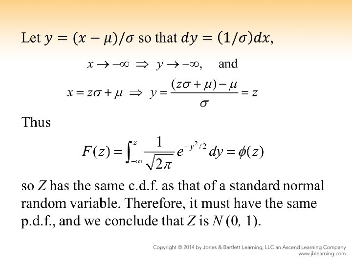
3. 4 – The Normal Distribution Definition 3. 4. 1 A continuous random variable Z has a standard normal distribution if its p. d. f. is

The c. d. f. See Table C. 1 – Two important properties

Example 3. 4. 1

The Normal Distribution •

The Normal Distribution

Empirical Rule

Relationship •

Application The “z-score” of x is

Example 3. 4. 2 •

Example 3. 4. 2 •

3. 5 – Functions of Continuous Random Variables Goal: To find the p. d. f. of a variable defined in terms of another variable – An important relationship – Second Fundamental Theorem of Calculus

Example 3. 5. 2 •

Joint pmf • The joint pmf of a the discrete random variables X and Y is • f(x, y)=P(X=x, Y=y)

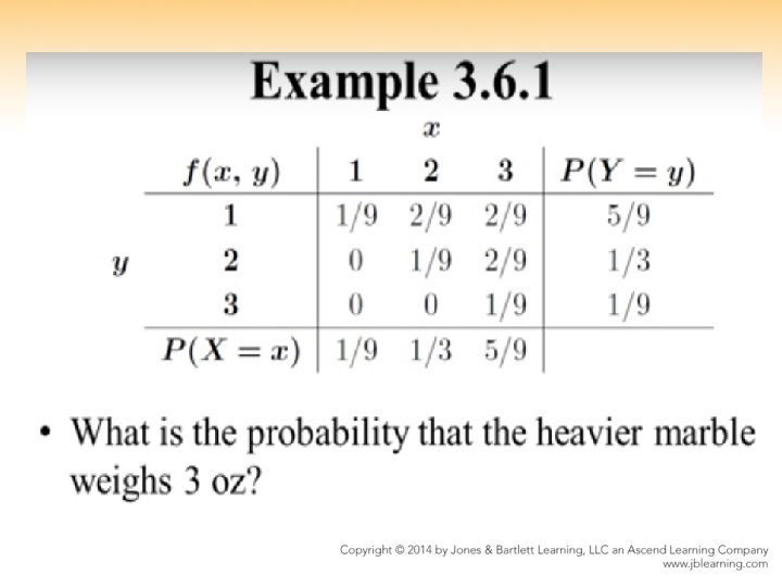
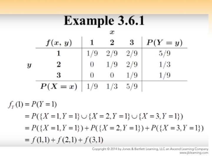
Example 3. 6. 1 • Bag contains 1 oz, 2 oz, and 3 oz marble • Random experiment – Choose 2 marbles with replacement • Sample space? • Let – X=weight of the heavier marble – Y=weight of the lighter marble
=P(X=1, Y=1)=P(M 1, M 1)=1/9 • f(2, 1)=")
Example 3. 6. 1 • f(1, 1)=P(X=1, Y=1)=P(M 1, M 1)=1/9 • f(2, 1)=
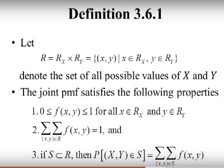

3. 6 – Joint Distributions Definition 3. 6. 2 Let X and Y be two continuous random variables. The joint probability density function, or joint p. d. f. , is an integrable function f(x, y) that satisfies the following three properties:

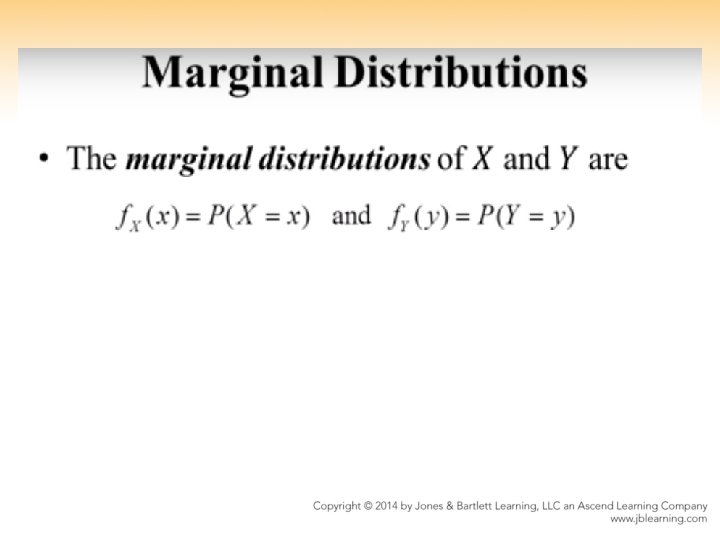
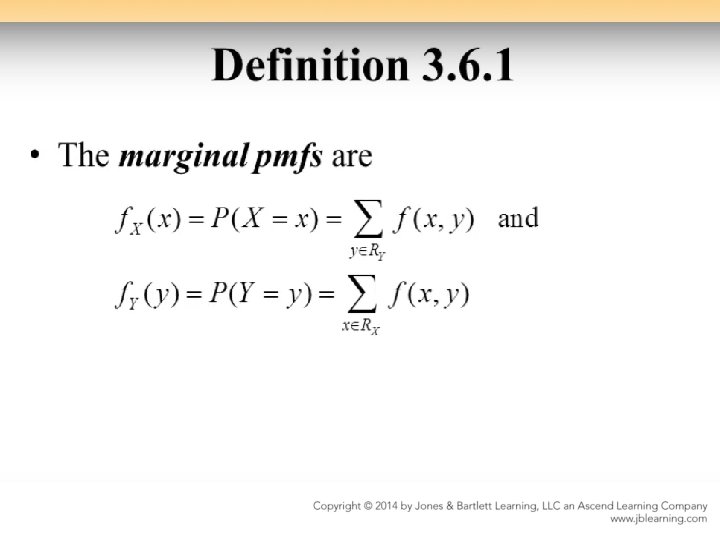
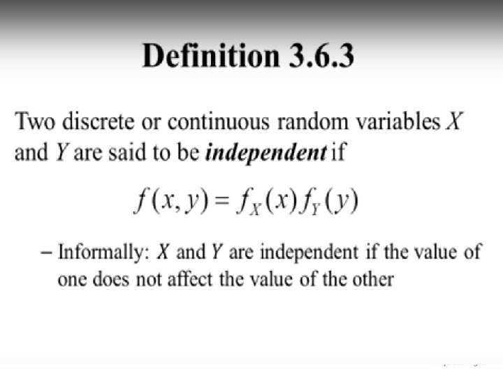
Marginal Distributions The marginal probability density functions, or marginal p. d. f. ’s, of X and Y are Definition 3. 6. 3 Two discrete or continuous random variables X and Y are said to be independent if

Example 3. 6. 3 Suppose the joint p. d. f. of X and Y is Note Marginal p. d. f. ’s:

Example 3. 6. 4 Suppose a man and a woman agree to meet at a restaurant sometime between 6: 00 and 6: 15 PM. Find the probability that the man has to wait longer than five minutes for the woman to arrive. – Let X and Y denote the number of minutes past 6: 00 PM that the man and the woman arrive, respectively.

Example 3. 6. 4 Assume Then

3. 7 – Functions of Independent Random Variables •

Example 3. 7. 1 Suppose the joint p. d. f. of X and Y is

Properties Theorem 3. 7. 1 For any discrete or continuous random variables, If X and Y are independent, then Theorem 3. 7. 2 If X and Y are independent, then

Properties •

Properties

Example 3. 7. 5 •
- Slides: 76