Chapter 3 Applications of Linear and Integer Programming

Chapter 3 Applications of Linear and Integer Programming Models - 2 1

3. 5 Applications of Integer Linear Programming Models Many real life problems call for at least one integer decision variable. n There are three types of Integer models: n Pure integer (AILP) n Mixed integer (MILP) n Binary (BILP) n 2

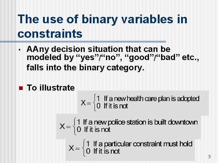
The use of binary variables in constraints • AAny decision situation that can be modeled by “yes”/“no”, “good”/“bad” etc. , falls into the binary category. n To illustrate 3

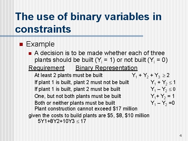
The use of binary variables in constraints n Example A decision is to be made whether each of three plants should be built (Yi = 1) or not built (Yi = 0) Requirement Binary Representation n At least 2 plants must be built Y 1 + Y 2 + Y 3 ³ 2 If plant 1 is built, plant 2 must not be built Y 1 + Y 2 £ 1 If plant 1 is built, plant 2 must be built Y 1 – Y 2 £ 0 One, but not both plants must be built Y 1 + Y 2 = 1 Both or neither plants must be built Y 1 – Y 2 =0 Plant construction cannot exceed $17 million given the costs to build plants are $5, $8, $10 million 5 Y 1+8 Y 2+10 Y 3 £ 17 4

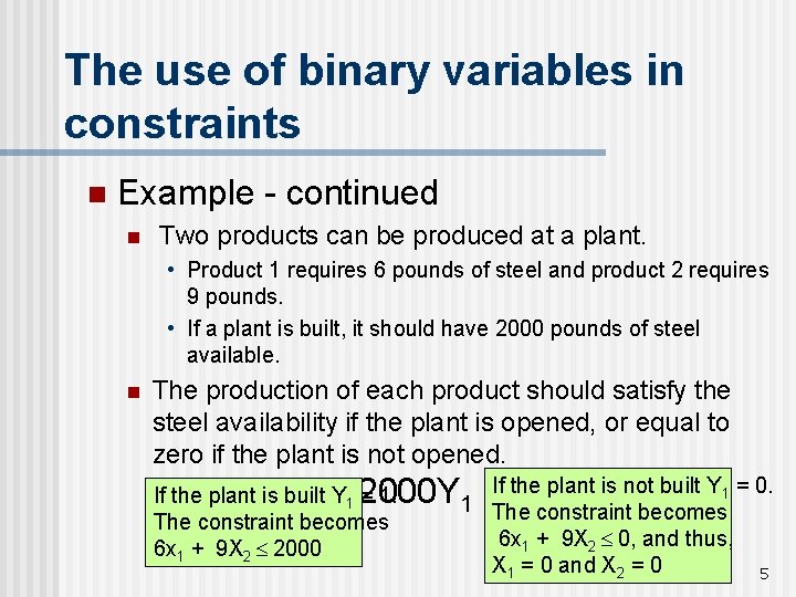
The use of binary variables in constraints n Example - continued n Two products can be produced at a plant. • Product 1 requires 6 pounds of steel and product 2 requires 9 pounds. • If a plant is built, it should have 2000 pounds of steel available. n The production of each product should satisfy the steel availability if the plant is opened, or equal to zero if the plant is not opened. 6 X + 9 X £ 2000 Y 1 If the plant is built 1 2 Y 1 = 1. The constraint becomes 6 x 1 + 9 X 2 £ 2000 If the plant is not built Y 1 = 0. The constraint becomes 6 x 1 + 9 X 2 £ 0, and thus, X 1 = 0 and X 2 = 0 5

3. 5. 1 Personnel Scheduling Models Assignments of personnel to jobs under minimum required coverage is a typical integer problems. n When resources are available over more than one period, linking constraint link the resources available in period t to the resources available in a period t+1. n 6

7

ul o oos k You look funny kso o s o l of u un ny Yo y n fun yy n nunn You look sofuffunny soo k o s lo k u o Y loo u o Y Yoouu l o l You look oook so funny k s so f u n o n y fu n n y 8

Sunset Beach Lifeguard Assignments n The City of Sunset Beach staffs lifeguards 7 days a week. n Regulations require that city employees work five days. n Insurance requirements mandate 1 lifeguard per 8000 average daily attendance on any given day. n The city wants to employ as few lifeguards as 9

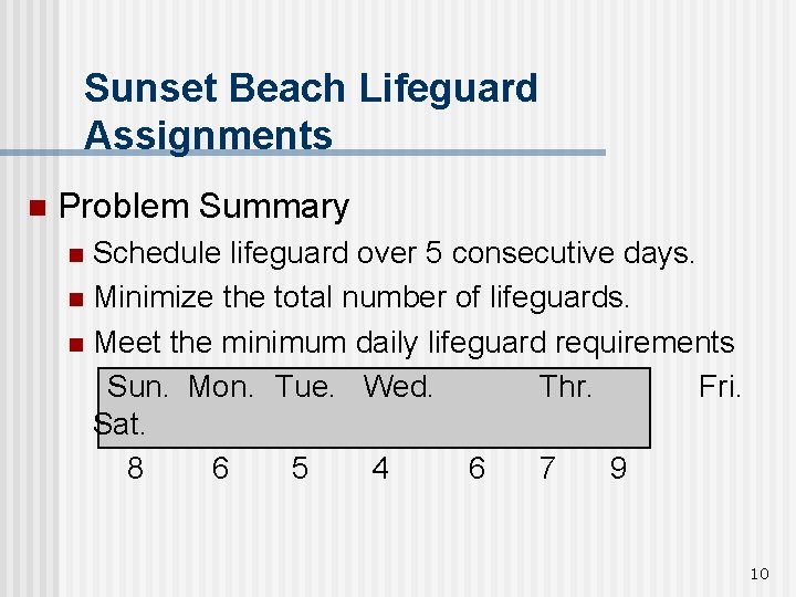
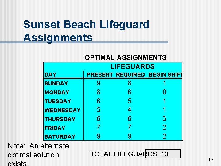
Sunset Beach Lifeguard Assignments n Problem Summary Schedule lifeguard over 5 consecutive days. n Minimize the total number of lifeguards. n Meet the minimum daily lifeguard requirements Sun. Mon. Tue. Wed. Thr. Fri. Sat. 8 6 5 4 6 7 9 n 10

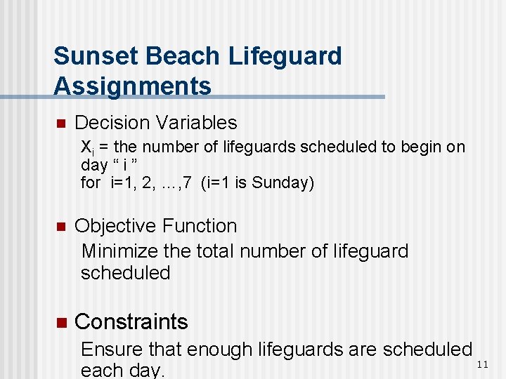
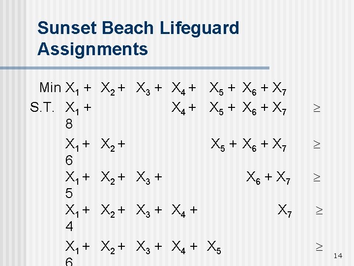
Sunset Beach Lifeguard Assignments n Decision Variables Xi = the number of lifeguards scheduled to begin on day “ i ” for i=1, 2, …, 7 (i=1 is Sunday) n Objective Function Minimize the total number of lifeguard scheduled n Constraints Ensure that enough lifeguards are scheduled 11 each day.

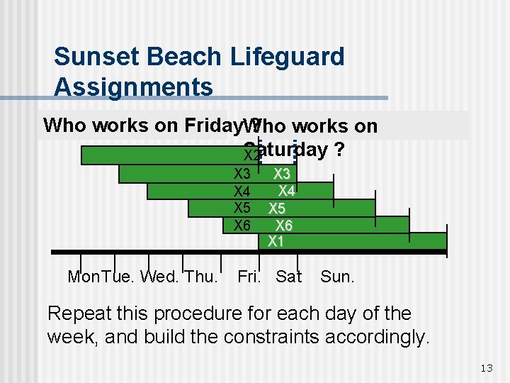
Sunset Beach Lifeguard Assignments To ensure that enough lifeguards are scheduled each day, identify which workers are on duty. For example: … 12

Sunset Beach Lifeguard Assignments Who works on Friday. Who ? works on Saturday ? X 2 X 3 X 4 X 5 X 6 Mon Tue. Wed. Thu. X 3 X 4 X 5 X 6 X 1 Fri. Sat Sun. Repeat this procedure for each day of the week, and build the constraints accordingly. 13

Sunset Beach Lifeguard Assignments Min X 1 + S. T. X 1 + 8 X 1 + 6 X 1 + 5 X 1 + 4 X 1 + X 2 + X 3 + X 4 + X 5 + X 6 + X 7 ³ X 2 + X 5 + X 6 + X 7 ³ X 2 + X 3 + X 4 + X 5 ³ 14

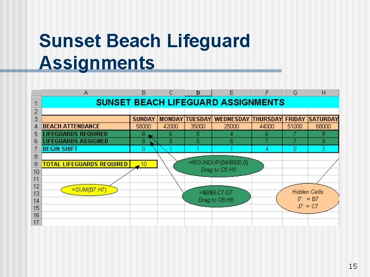
Sunset Beach Lifeguard Assignments 15

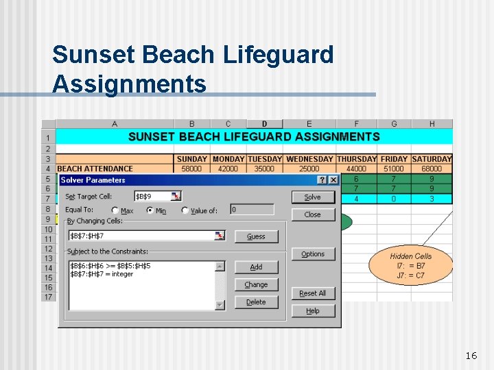
Sunset Beach Lifeguard Assignments 16

Sunset Beach Lifeguard Assignments OPTIMAL ASSIGNMENTS LIFEGUARDS DAY SUNDAY MONDAY TUESDAY WEDNESDAY THURSDAY FRIDAY SATURDAY Note: An alternate optimal solution PRESENT REQUIRED BEGIN SHIFT 9 8 6 5 6 7 9 8 6 5 4 6 7 9 1 0 1 1 3 2 2 TOTAL LIFEGUARDS 10 17

3. 5. 2 Project selection Models These models involve a “go/no-go” situations, that can be modeled using binary variables. n Typical elements in such models are: n Budget n Space n Priority conditions n 18

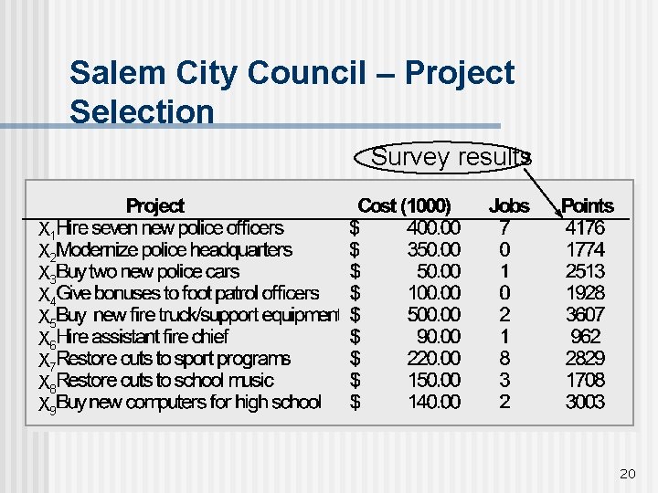
Salem City Council – Project Selection The Salem City Council needs to decide how to allocate funds to nine projects such that public support is maximized. n Data reflect costs, resource availabilities, concerns and priorities the city council has. n 19

Salem City Council – Project Selection Survey results X 1 X 2 X 3 X 4 X 5 X 6 X 7 X 8 X 9 20

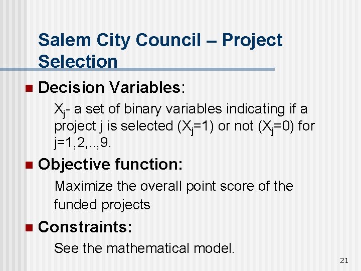
Salem City Council – Project Selection n Decision Variables: Xj- a set of binary variables indicating if a project j is selected (Xj=1) or not (Xj=0) for j=1, 2, . . , 9. n Objective function: Maximize the overall point score of the funded projects n Constraints: See the mathematical model. 21

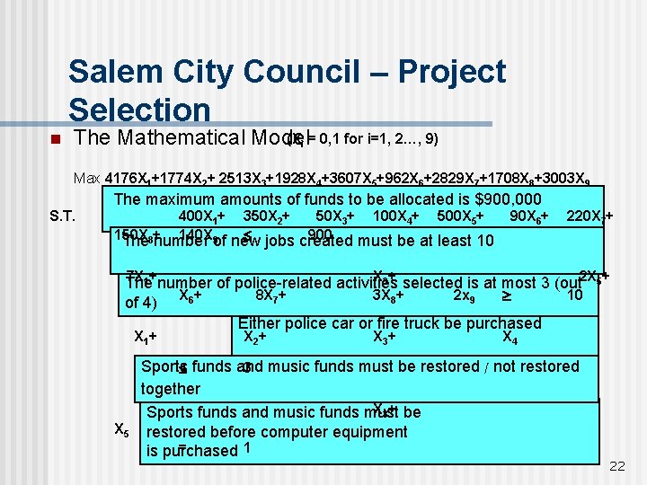
Salem City Council – Project Selection n (Xi = 0, 1 for i=1, 2…, 9) The Mathematical Model Max 4176 X 1+1774 X 2+ 2513 X 3+1928 X 4+3607 X 5+962 X 6+2829 X 7+1708 X 8+3003 X 9 S. T. The maximum amounts of funds to be allocated is $900, 000 400 X 1+ 350 X 2+ 50 X 3+ 100 X 4+ 500 X 5+ 150 X 140 X 9 of new £ jobs created 900 The 8+number must be at least 10 90 X 6+ 220 X 7+ 7 X 1+ X 3+ The number of police-related activities selected is at most 3 (out 2 X 5+ 8 X 7+ 3 X 8+ 2 x 9 ³ 10 of 4) X 6+ Either police car or fire truck be purchased X 1+ X 5 X 2+ X 3+ X 4 Sports £ funds and 3 music funds must be restored / not restored together X 3+ be Sports funds and music funds must restored before computer equipment = 1 is purchased 22

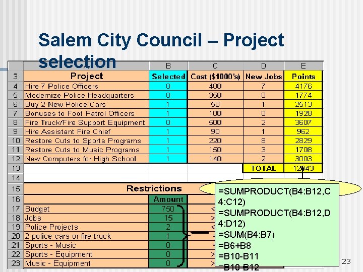
Salem City Council – Project selection =SUMPRODUCT(B 4: B 12, C E 4: E 12) 4: C 12) =SUMPRODUCT(B 4: B 12, D 4: D 12) =SUM(B 4: B 7) =B 6+B 8 =B 10 -B 11 =B 10 -B 12 23

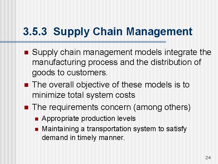
3. 5. 3 Supply Chain Management n n n Supply chain management models integrate the manufacturing process and the distribution of goods to customers. The overall objective of these models is to minimize total system costs The requirements concern (among others) n n Appropriate production levels Maintaining a transportation system to satisfy demand in timely manner. 24

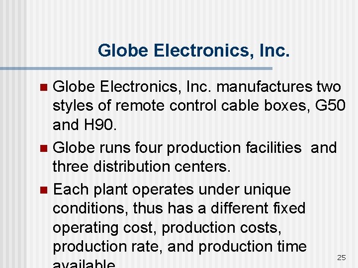
Globe Electronics, Inc. manufactures two styles of remote control cable boxes, G 50 and H 90. n Globe runs four production facilities and three distribution centers. n Each plant operates under unique conditions, thus has a different fixed operating cost, production costs, production rate, and production time n 25

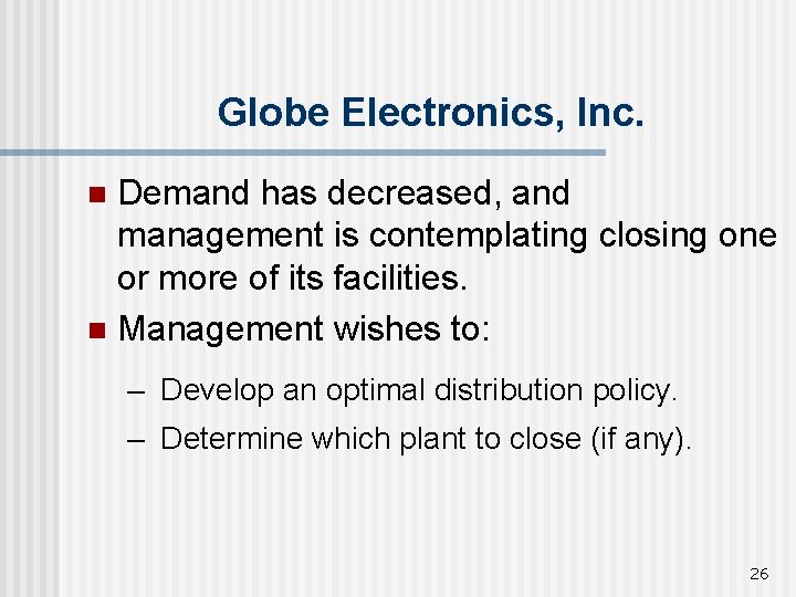
Globe Electronics, Inc. Demand has decreased, and management is contemplating closing one or more of its facilities. n Management wishes to: n – Develop an optimal distribution policy. – Determine which plant to close (if any). 26

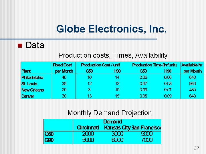
Globe Electronics, Inc. n Data Production costs, Times, Availability Monthly Demand Projection 27

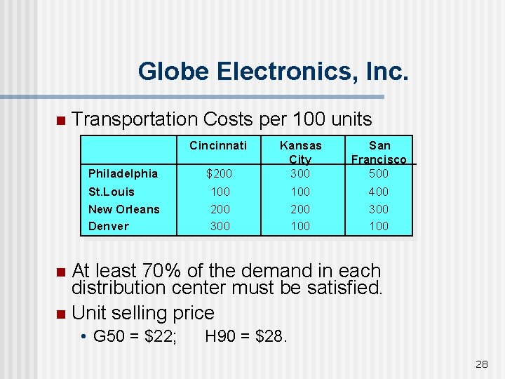
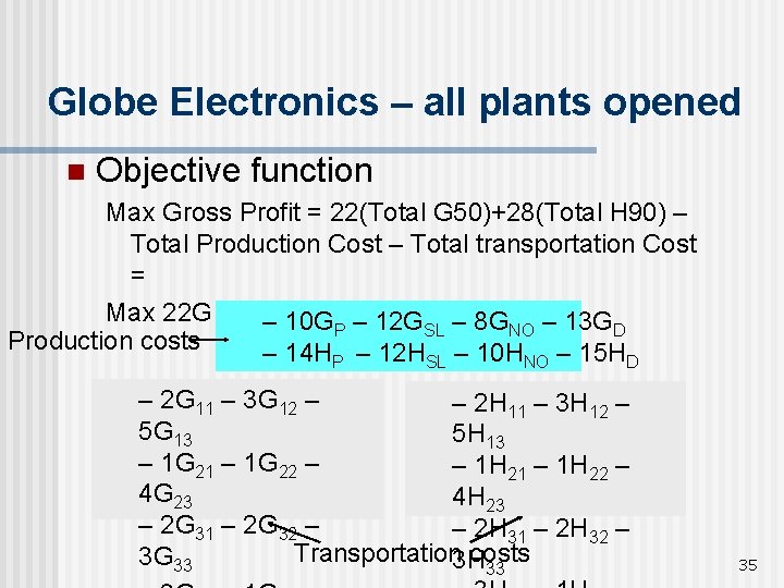
Globe Electronics, Inc. n Transportation Costs per 100 units Cincinnati Philadelphia $200 Kansas City 300 St. Louis New Orleans Denver 100 200 300 100 200 100 San Francisco 500 400 300 100 At least 70% of the demand in each distribution center must be satisfied. n Unit selling price n • G 50 = $22; H 90 = $28. 28

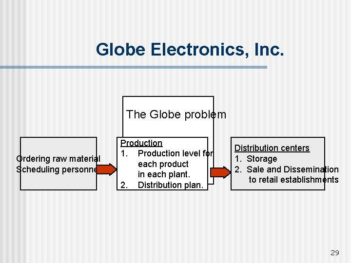
Globe Electronics, Inc. The Globe problem Ordering raw material Scheduling personnel Production 1. Production level for each product in each plant. 2. Distribution plan. Distribution centers 1. Storage 2. Sale and Dissemination to retail establishments 29

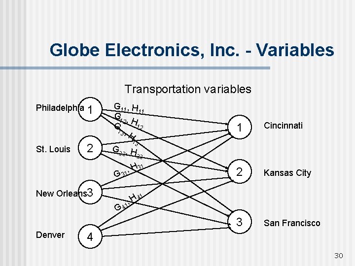
Globe Electronics, Inc. - Variables Transportation variables Philadelphia 1 St. Louis 2 G 11, H 11 G 2 , H 12 13 , H Cincinnati 2 Kansas City 3 San Francisco 13 G 22 , H 22 , 1 H 31 G 3 New Orleans 3 1 1 , 1 H 4 G 4 Denver 4 30

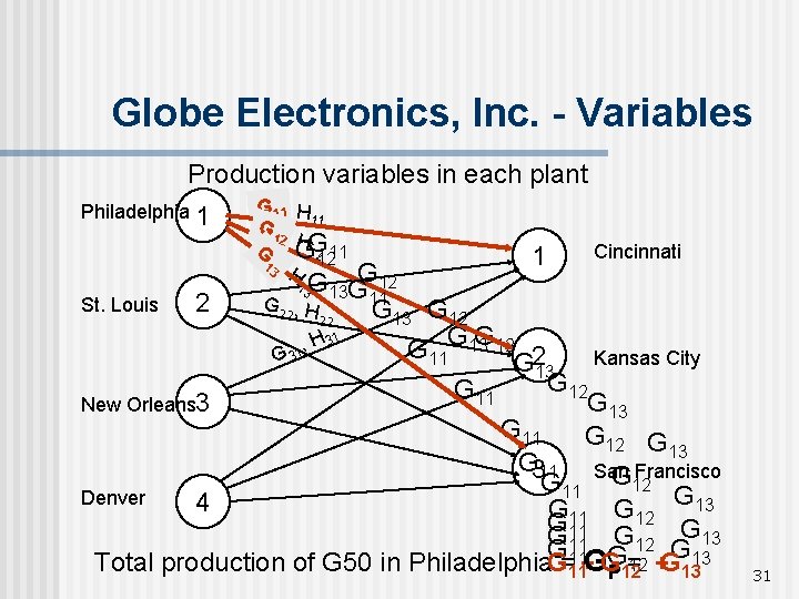
Globe Electronics, Inc. - Variables Production variables in each plant Philadelphia 1 G 1111, H 11 G 11 , H G G 22 G 1 2 11 12 13 , H 1 Cincinnati G 13 GG 1112 G 22 , H 2 St. Louis G 13 G 12 22 G 13 G 12 , H 31 G 3 11 G 213 Kansas City G 12 G 11 G 13 New Orleans 3 G 11 G 12 G 13 G 311 San Francisco G 11 G 12 G 13 Denver 4 G G 11 12 G 11 G 13 G G 11 12 G 13 G Total production of G 50 in Philadelphia. G G = G=11 + G 12 + G 11 P 12 13 13 31

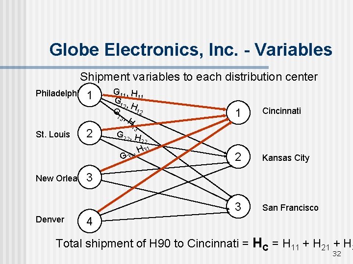
Globe Electronics, Inc. - Variables Shipment variables to each distribution center Philadelphia 1 St. Louis 2 G 11, H 11 G 1 , G 2 H 12 13 , H 1 Cincinnati 2 Kansas City 3 San Francisco 13 G 22 , H 31 G 31 New Orleans 3 Denver 4 Total shipment of H 90 to Cincinnati = HC = H 11 + H 21 + H 3 32

Globe Electronics Model No. 1: All The Plants Remain Operational 33

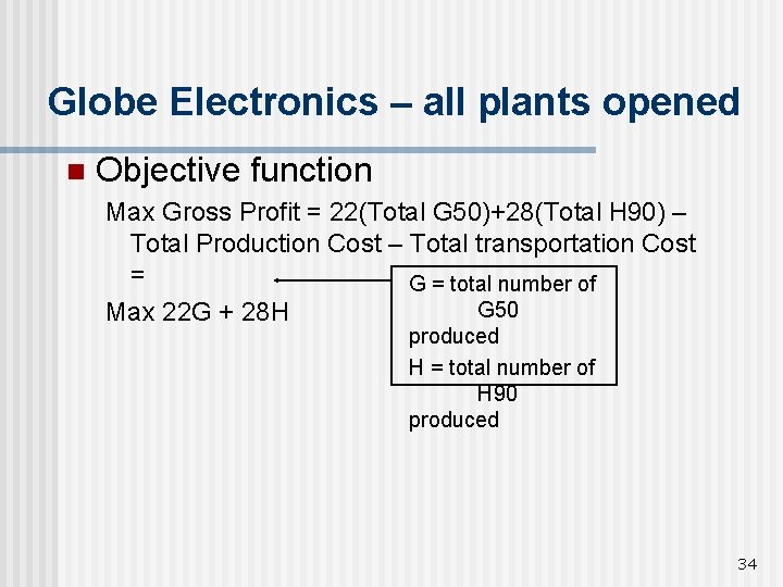
Globe Electronics – all plants opened n Objective function Max Gross Profit = 22(Total G 50)+28(Total H 90) – Total Production Cost – Total transportation Cost = G = total number of G 50 Max 22 G + 28 H produced H = total number of H 90 produced 34

Globe Electronics – all plants opened n Objective function Max Gross Profit = 22(Total G 50)+28(Total H 90) – Total Production Cost – Total transportation Cost = Max 22 G + 28 H – 10 GP – 12 GSL – 8 GNO – 13 GD Production costs – 14 H – 12 H – 10 H – 15 H P SL NO D – 2 G 11 – 3 G 12 – – 2 H 11 – 3 H 12 – 5 G 13 5 H 13 – 1 G 21 – 1 G 22 – – 1 H 21 – 1 H 22 – 4 G 23 4 H 23 – 2 G 31 – 2 G 32 – – 2 H 31 – 2 H 32 – Transportation 3 H costs 3 G 33 33 35

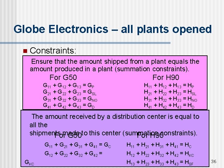
Globe Electronics – all plants opened n Constraints: Ensure that the amount shipped from a plant equals the amount produced in a plant (summation constraints). For G 50 G 11 + G 12 + G 13 = GP G 21 + G 22 + G 23 = GSL G 31 + G 32 + G 33 = GNO G 41 + G 42 + G 43 = GD For H 90 H 11 + H 12 + H 13 = HP H 21 + H 22 + H 23 = HSL H 31 + H 32 + H 33 = HNO H 41 + H 42 + H 43 = HD The amount received by a distribution center is equal to all the shipments Formade G 50 to this center (summation For H 90 constraints). GKC G 11 + G 21 + G 31 + G 41 = GC H 11 + H 21 + H 31 + H 41 = HC G 12 + G 22 + G 32 + G 42 = H 12 + H 22 + H 32 + H 42 = HKC H 13 + H 23 + H 33 + H 43 = HSF 36

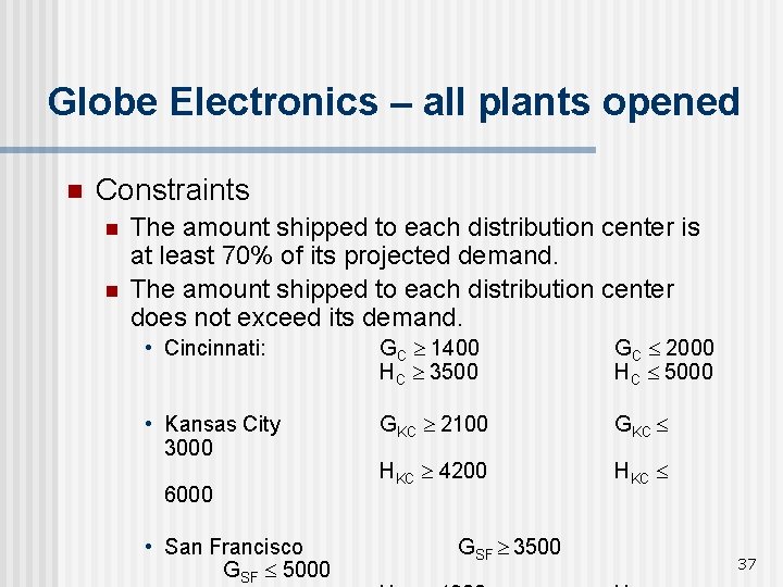
Globe Electronics – all plants opened n Constraints n n The amount shipped to each distribution center is at least 70% of its projected demand. The amount shipped to each distribution center does not exceed its demand. • Cincinnati: GC ³ 1400 HC ³ 3500 GC £ 2000 HC £ 5000 • Kansas City 3000 GKC ³ 2100 GKC £ HKC ³ 4200 HKC £ 6000 • San Francisco GSF £ 5000 GSF ³ 3500 37

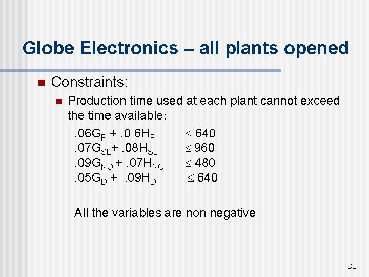
Globe Electronics – all plants opened n Constraints: n Production time used at each plant cannot exceed the time available: . 06 GP +. 0 6 HP £ 640. 07 GSL+. 08 HSL £ 960. 09 GNO +. 07 HNO £ 480. 05 GD +. 09 HD £ 640 All the variables are non negative 38

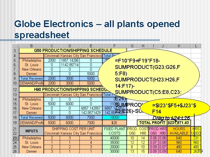
Globe Electronics – all plants opened spreadsheet =F 10*F 9+F 19*F 18 SUMPRODUCT(G 23: G 26, F 5: F 8) SUMPRODUCT(H 23: H 26, F 14: F 17)SUMPRODUCT(C 5: E 8, C 23: E 26)SUMPRODUCT(C 14: E 17, C =$I 23*$F 5+$J 23*$ 23: E 26)-SUM(F 23: F 26) F 14 Drag to L 24: L 26 39

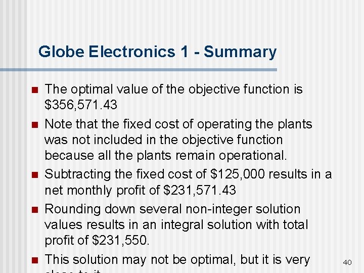
Globe Electronics 1 - Summary n n n The optimal value of the objective function is $356, 571. 43 Note that the fixed cost of operating the plants was not included in the objective function because all the plants remain operational. Subtracting the fixed cost of $125, 000 results in a net monthly profit of $231, 571. 43 Rounding down several non-integer solution values results in an integral solution with total profit of $231, 550. This solution may not be optimal, but it is very 40

Globe Electronics Model No. 2: The number of plants that remain operational in each city is a decision variable. 41

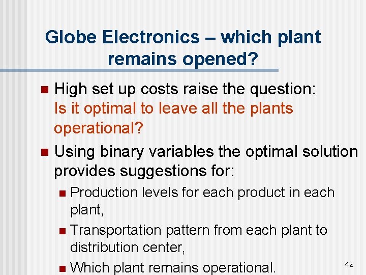
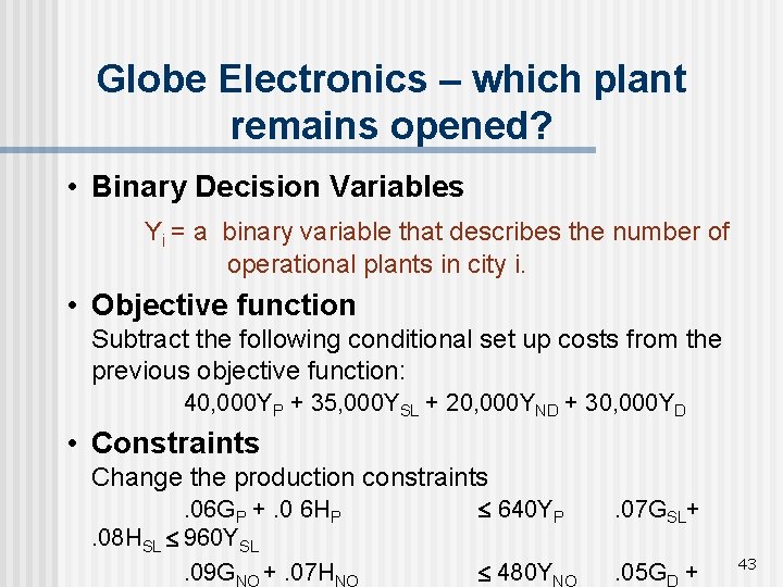
Globe Electronics – which plant remains opened? High set up costs raise the question: Is it optimal to leave all the plants operational? n Using binary variables the optimal solution provides suggestions for: n Production levels for each product in each plant, n Transportation pattern from each plant to distribution center, n Which plant remains operational. n 42

Globe Electronics – which plant remains opened? • Binary Decision Variables Yi = a binary variable that describes the number of operational plants in city i. • Objective function Subtract the following conditional set up costs from the previous objective function: 40, 000 YP + 35, 000 YSL + 20, 000 YND + 30, 000 YD • Constraints Change the production constraints. 06 GP +. 0 6 HP. 08 HSL £ 960 YSL. 09 GNO +. 07 HNO £ 640 YP . 07 GSL+ £ 480 YNO . 05 GD + 43

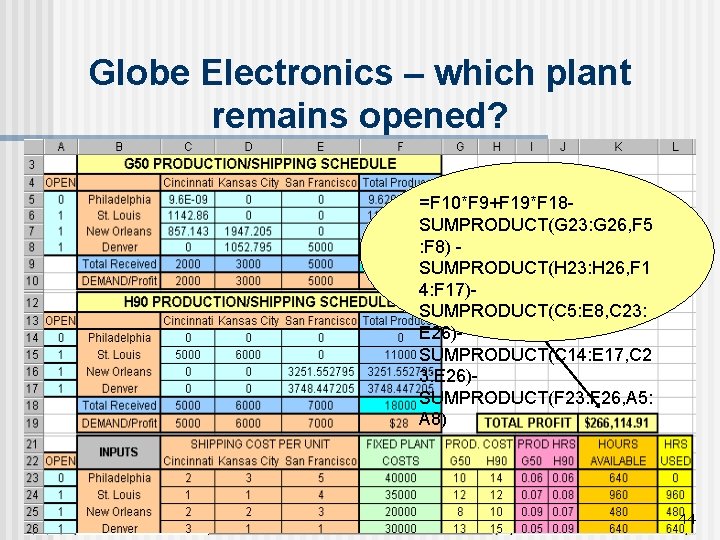
Globe Electronics – which plant remains opened? =F 10*F 9+F 19*F 18 SUMPRODUCT(G 23: G 26, F 5 : F 8) SUMPRODUCT(H 23: H 26, F 1 4: F 17)SUMPRODUCT(C 5: E 8, C 23: E 26)SUMPRODUCT(C 14: E 17, C 2 3: E 26)SUMPRODUCT(F 23: F 26, A 5: A 8) 44

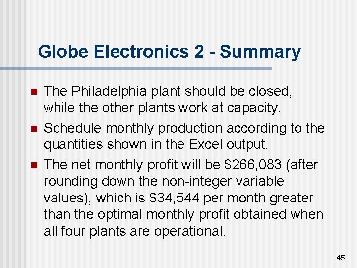
Globe Electronics 2 - Summary n n n The Philadelphia plant should be closed, while the other plants work at capacity. Schedule monthly production according to the quantities shown in the Excel output. The net monthly profit will be $266, 083 (after rounding down the non-integer variable values), which is $34, 544 per month greater than the optimal monthly profit obtained when all four plants are operational. 45

Appendix 3. 4 (CD): Advertising Models 46

Appendix 3. 4 (CD): Advertising Models n n Many marketing situations can be modeled by linear programming models. Typically, such models consist of: n n n Budget constraints, Deadlines constraints, Choice of media, Exposure to target population. The objective is to achieve the most effective advertising plan. 47

Vertex Software, Inc. n Vertex Software has developed a new software product, LUMBER 2000. n A marketing plan for this product is to be developed for the next quarter. n n The product will be promoted using black and white and colored full page ads. Three publications are considered: • Building Today • Lumber Weekly • Timber World 48

Vertex Software, Inc. n Requirements n A maximum of one ad should be placed in any one issue of any of the publication during the quarter. n At least 50 full-page ads should appear during the quarter. n at least 8 color ads should appear during the quarter. n One ad should appear in each issue of Timber World. n At least 4 weeks of advertising should be placed in each of the Building Today and Lumber Weekly publications. n No more than $ 40000 should be spent on advertising 49

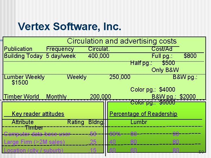
Vertex Software, Inc. Circulation and advertising costs Publication Frequency Building Today 5 day/week Lumber Weekly $1500 Timber World Circulat. 400, 000 Cost/Ad Full pg. : $800 Half pg. : $500 Only B&W 250, 000 B&W pg. : Weekly Monthly Key reader attitudes Attribute Rating Timber Computer data-base user Large Firm (>2 M sales) Location (city / suburb) 200, 000 Color pg. : $4000 B&W pg. : $2000 Color pg. : $6000 Percentage of Readership Bldng. Lumbr. 50. 25. 15 60% 40 60 80 80 60 90 80 80 50

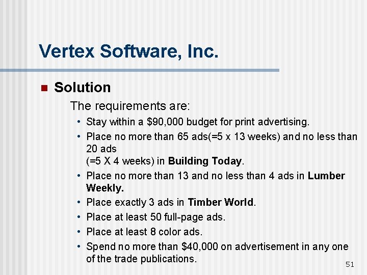
Vertex Software, Inc. n Solution The requirements are: • Stay within a $90, 000 budget for print advertising. • Place no more than 65 ads(=5 x 13 weeks) and no less than 20 ads (=5 X 4 weeks) in Building Today. • Place no more than 13 and no less than 4 ads in Lumber Weekly. • Place exactly 3 ads in Timber World. • Place at least 50 full-page ads. • Place at least 8 color ads. • Spend no more than $40, 000 on advertisement in any one of the trade publications. 51

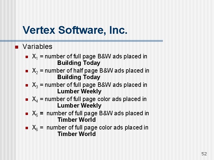
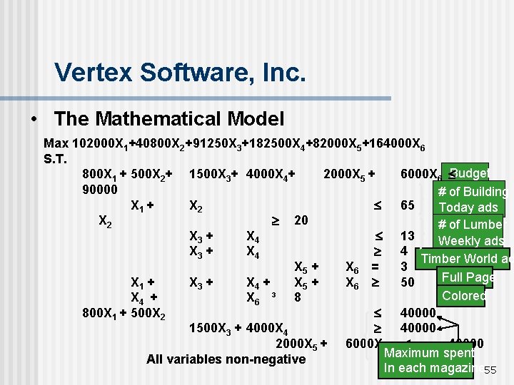
Vertex Software, Inc. n Variables n n n X 1 = number of full page B&W ads placed in Building Today X 2 = number of half page B&W ads placed in Building Today X 3 = number of full page B&W ads placed in Lumber Weekly X 4 = number of full page color ads placed in Lumber Weekly X 5 = number of full page B&W ads placed in Timber World X 6 = number of full page color ads placed in Timber World 52

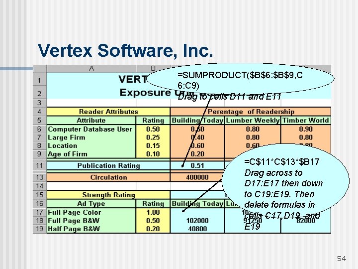
Vertex Software, Inc. n The Objective Function n The objective function measures the effectiveness of the promotion operation (to be maximized). n It depends on the number of ads in each publication, as well as on the relative effectiveness per ad. n A special technique (external to this problem) is applied to evaluate this relative effectiveness. 53

Vertex Software, Inc. =SUMPRODUCT($B$6: $B$9, C 6: C 9) Drag to cells D 11 and E 11 =C$11*C$13*$B 17 Drag across to D 17: E 17 then down to C 19: E 19. Then delete formulas in cells C 17, D 19, and E 19 54

Vertex Software, Inc. • The Mathematical Model Max 102000 X 1+40800 X 2+91250 X 3+182500 X 4+82000 X 5+164000 X 6 S. T. 800 X 1 + 500 X 2+ 1500 X 3+ 4000 X 4+ 2000 X 5 + 6000 X 6 £Budget 90000 # of Building X 1 + X 2 £ 65 X 1 +ads Today X 2 ³ 20 # of Lumber X 3 + X 4 £ 13 Weekly ads X 3 + X 4 ³ 4 Timber World ad X 5 + X 6 = 3 Full Page X 1 + X 3 + X 4 + X 5 + X 6 ³ 50 Colored X 4 + X 6 ³ 8 800 X 1 + 500 X 2 £ 40000 1500 X 3 + 4000 X 4 ³ 40000 2000 X 5 + 6000 X 6 £ 40000 Maximum spent All variables non-negative In each magazine 55

Vertex Software, Inc. 56

Copyright �� 2002�John Wiley & Sons, Inc. All rights reserved. Reproduction or translation of this work beyond that named in Section 117 of the United States Copyright Act without the express written consent of the copyright owner is unlawful. Requests for further information should be addressed to the Permissions Department, John Wiley & Sons, Inc. Adopters of the textbook are granted permission to make back-up copies for their own use only, to make copies for distribution to students of the course the textbook is used in, and to modify this material to best suit their instructional needs. Under no circumstances can copies be made for resale. The Publisher assumes no responsibility for errors, omissions, or damages, caused by the use of these programs or from the use of the information contained herein. 57