CHAPTER 3 Analysis of Variance ANOVA PART 3

CHAPTER 3 Analysis of Variance (ANOVA) PART 3 = TWO-WAY ANOVA WITH REPLICATION (FACTORIAL EXPERIMENT) MADAM SITI AISYAH ZAKARIA EQT 271 SEM 2 2014/2015

Two-Way ANOVA with Replication (Factorial Experiment) • Factorial experiments and their corresponding ANOVA computations are valuable designs when simultaneous conclusions about two or more independent variable /factors are required. • In addition, any significance interaction between the factors will be investigated. • Replication means an independent variable repeat of each factor combination. (interaction effect) • Purpose: Examines (1) the effects of the interactions between different levels of the two factors on the dependent variable , y. (2) the effect of Factor A on the dependent variable, y; along with (3) the effect of Factor B on the dependent variable, y

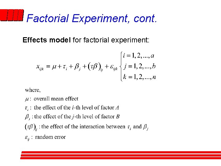
Factorial Experiment, cont. Effects model for factorial experiment:

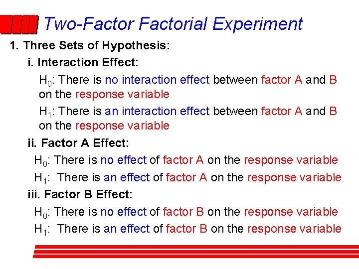
Two-Factorial Experiment 1. Three Sets of Hypothesis: i. Interaction Effect: H 0: There is no interaction effect between factor A and B on the response variable H 1: There is an interaction effect between factor A and B on the response variable ii. Factor A Effect: H 0: There is no effect of factor A on the response variable H 1: There is an effect of factor A on the response variable iii. Factor B Effect: H 0: There is no effect of factor B on the response variable H 1: There is an effect of factor B on the response variable

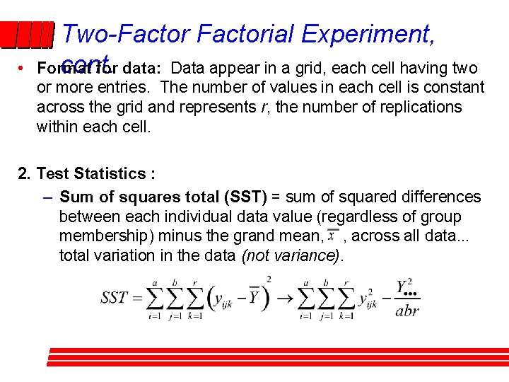
• Two-Factorial Experiment, cont. Format for data: Data appear in a grid, each cell having two or more entries. The number of values in each cell is constant across the grid and represents r, the number of replications within each cell. 2. Test Statistics : – Sum of squares total (SST) = sum of squared differences between each individual data value (regardless of group membership) minus the grand mean, , across all data. . . total variation in the data (not variance).

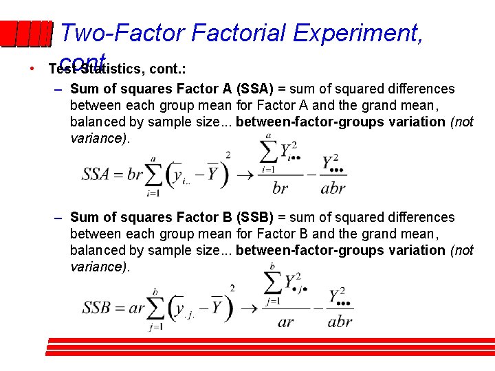
• Two-Factorial Experiment, cont. Test Statistics, cont. : – Sum of squares Factor A (SSA) = sum of squared differences between each group mean for Factor A and the grand mean, balanced by sample size. . . between-factor-groups variation (not variance). – Sum of squares Factor B (SSB) = sum of squared differences between each group mean for Factor B and the grand mean, balanced by sample size. . . between-factor-groups variation (not variance).

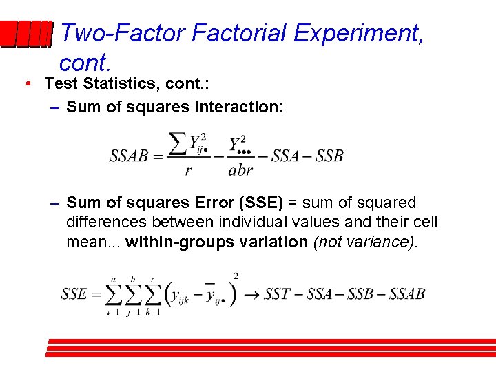
Two-Factorial Experiment, cont. • Test Statistics, cont. : – Sum of squares Interaction: – Sum of squares Error (SSE) = sum of squared differences between individual values and their cell mean. . . within-groups variation (not variance).

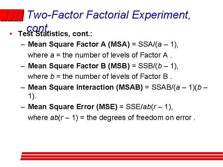
• Two-Factorial Experiment, cont. Test Statistics, cont. : – Mean Square Factor A (MSA) = SSA/(a – 1), where a = the number of levels of Factor A. – Mean Square Factor B (MSB) = SSB/(b – 1), where b = the number of levels of Factor B. – Mean Square Interaction (MSAB) = SSAB/(a – 1)(b – 1). – Mean Square Error (MSE) = SSE/ab(r – 1), where ab(r – 1) = the degrees of freedom on error.

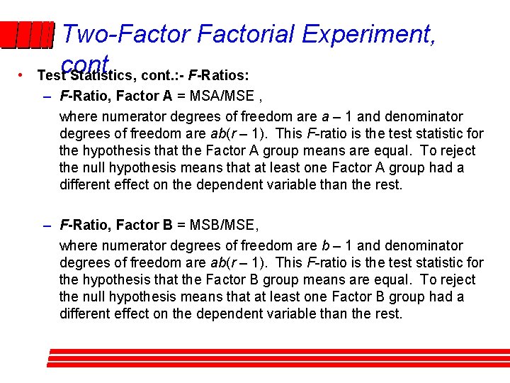
• Two-Factorial Experiment, Testcont. Statistics, cont. : - F-Ratios: – F-Ratio, Factor A = MSA/MSE , where numerator degrees of freedom are a – 1 and denominator degrees of freedom are ab(r – 1). This F-ratio is the test statistic for the hypothesis that the Factor A group means are equal. To reject the null hypothesis means that at least one Factor A group had a different effect on the dependent variable than the rest. – F-Ratio, Factor B = MSB/MSE, where numerator degrees of freedom are b – 1 and denominator degrees of freedom are ab(r – 1). This F-ratio is the test statistic for the hypothesis that the Factor B group means are equal. To reject the null hypothesis means that at least one Factor B group had a different effect on the dependent variable than the rest.

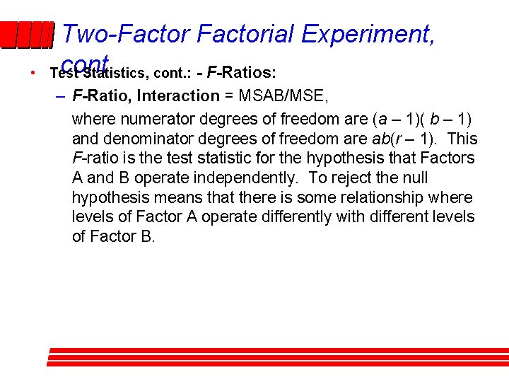
• Two-Factorial Experiment, cont. Test Statistics, cont. : - F-Ratios: – F-Ratio, Interaction = MSAB/MSE, where numerator degrees of freedom are (a – 1)( b – 1) and denominator degrees of freedom are ab(r – 1). This F-ratio is the test statistic for the hypothesis that Factors A and B operate independently. To reject the null hypothesis means that there is some relationship where levels of Factor A operate differently with different levels of Factor B.

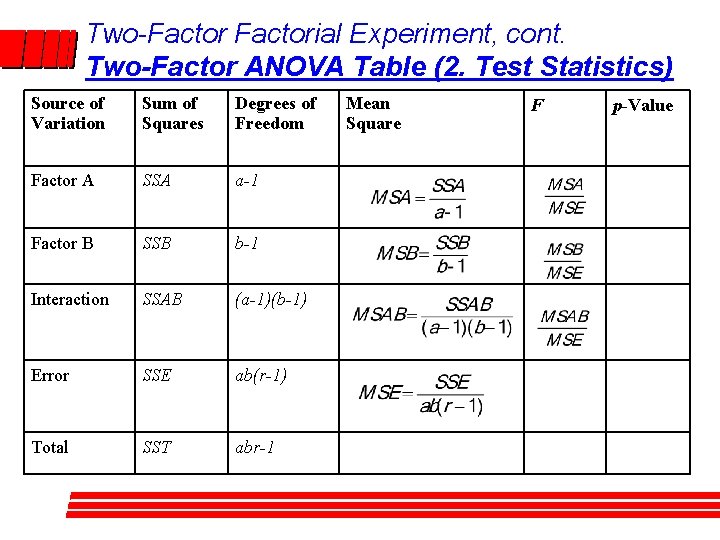
Two-Factorial Experiment, cont. Two-Factor ANOVA Table (2. Test Statistics) Source of Variation Sum of Squares Degrees of Freedom Factor A SSA a-1 Factor B SSB b-1 Interaction SSAB (a-1)(b-1) Error SSE ab(r-1) Total SST abr-1 Mean Square F p-Value

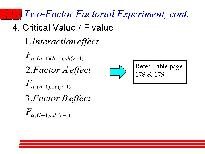
Two-Factorial Experiment, cont. 4. Critical Value / F value Refer Table page 178 & 179

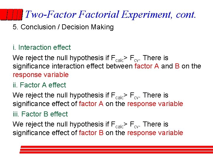
Two-Factorial Experiment, cont. 5. Conclusion / Decision Making i. Interaction effect We reject the null hypothesis if Fcalc> Fcv. There is significance interaction effect between factor A and B on the response variable ii. Factor A effect We reject the null hypothesis if Fcalc> Fcv. There is significance effect of factor A on the response variable iii. Factor B effect We reject the null hypothesis if Fcalc> Fcv. There is significance effect of factor B on the response variable

Two-Factorial Experiment, Example 4. 4: State of Ohio Wage Survey A survey was conducted of hourly wages for a sample of workers in two industries at three locations in Kedah. Part of the purpose of the survey was to determine if differences exist (an effect) in both industry type and location. The sample data are shown on the next slide.

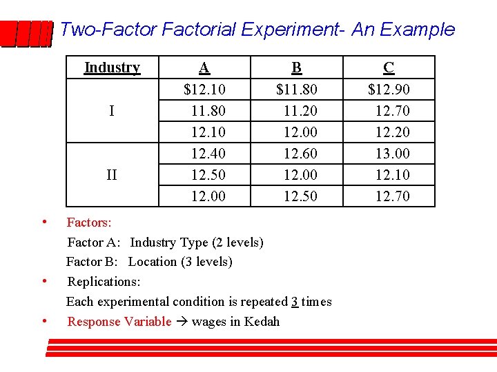
Two-Factorial Experiment- An Example Industry I II • • • A $12. 10 11. 80 12. 10 12. 40 12. 50 12. 00 B $11. 80 11. 20 12. 00 12. 60 12. 00 12. 50 Factors: Factor A: Industry Type (2 levels) Factor B: Location (3 levels) Replications: Each experimental condition is repeated 3 times Response Variable wages in Kedah C $12. 90 12. 70 12. 20 13. 00 12. 10 12. 70

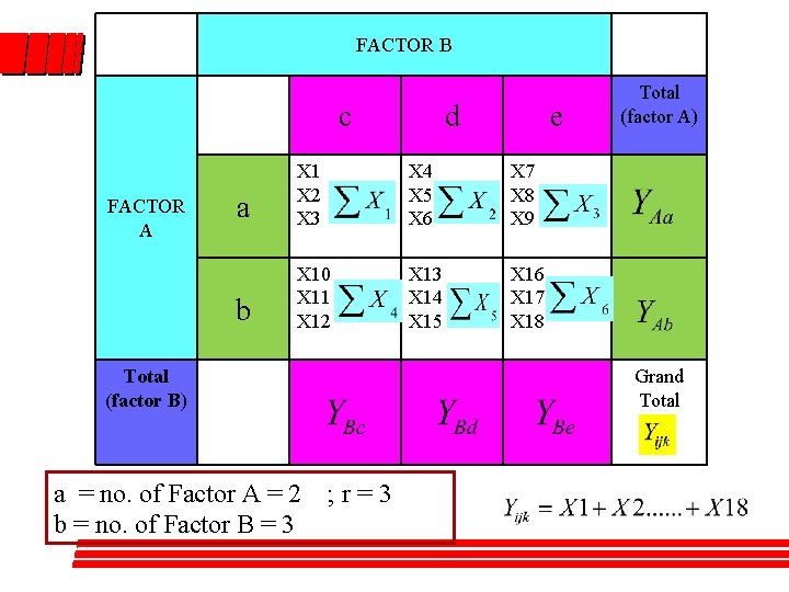
FACTOR B c FACTOR A d e a X 1 X 2 X 3 X 4 X 5 X 6 X 7 X 8 X 9 b X 10 X 11 X 12 X 13 X 14 X 15 X 16 X 17 X 18 Total (factor B) a = no. of Factor A = 2 b = no. of Factor B = 3 Total (factor A) Grand Total ; r=3

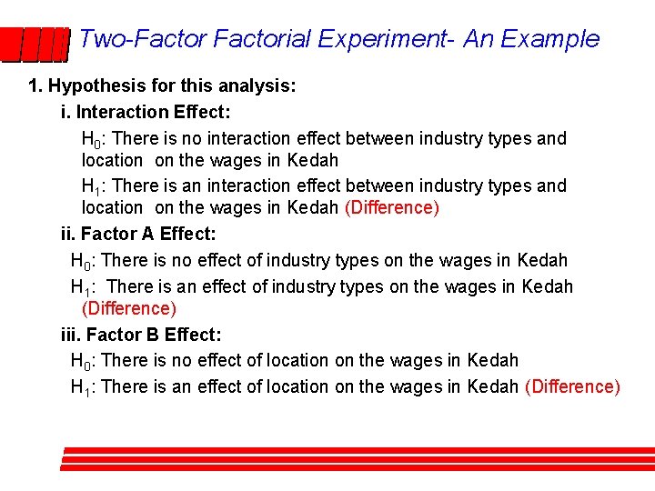
Two-Factorial Experiment- An Example 1. Hypothesis for this analysis: i. Interaction Effect: H 0: There is no interaction effect between industry types and location on the wages in Kedah H 1: There is an interaction effect between industry types and location on the wages in Kedah (Difference) ii. Factor A Effect: H 0: There is no effect of industry types on the wages in Kedah H 1: There is an effect of industry types on the wages in Kedah (Difference) iii. Factor B Effect: H 0: There is no effect of location on the wages in Kedah H 1: There is an effect of location on the wages in Kedah (Difference)

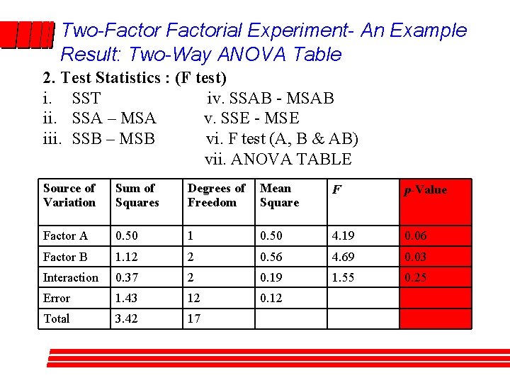
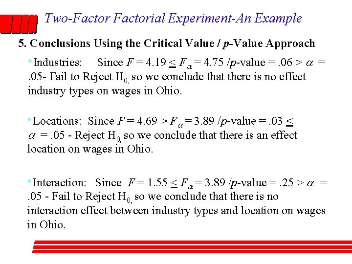
Two-Factorial Experiment- An Example Result: Two-Way ANOVA Table 2. Test Statistics : (F test) i. SST iv. SSAB - MSAB ii. SSA – MSA v. SSE - MSE iii. SSB – MSB vi. F test (A, B & AB) vii. ANOVA TABLE Source of Variation Sum of Squares Degrees of Freedom Mean Square F p-Value Factor A 0. 50 1 0. 50 4. 19 0. 06 Factor B 1. 12 2 0. 56 4. 69 0. 03 Interaction 0. 37 2 0. 19 1. 55 0. 25 Error 1. 43 12 0. 12 Total 3. 42 17

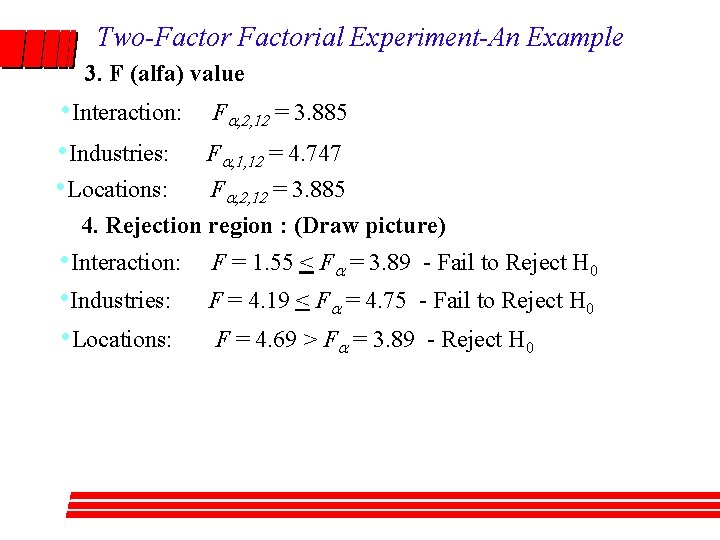
Two-Factorial Experiment-An Example 3. F (alfa) value • Interaction: • Industries: • Locations: Fa, 2, 12 = 3. 885 Fa, 1, 12 = 4. 747 Fa, 2, 12 = 3. 885 4. Rejection region : (Draw picture) • Interaction: • Industries: • Locations: F = 1. 55 < Fa = 3. 89 - Fail to Reject H 0 F = 4. 19 < Fa = 4. 75 - Fail to Reject H 0 F = 4. 69 > Fa = 3. 89 - Reject H 0

Two-Factorial Experiment-An Example 5. Conclusions Using the Critical Value / p-Value Approach • Industries: Since F = 4. 19 < Fa = 4. 75 /p-value =. 06 > a =. 05 - Fail to Reject H 0, so we conclude that there is no effect industry types on wages in Ohio. • Locations: Since F = 4. 69 > Fa = 3. 89 /p-value =. 03 < a =. 05 - Reject H 0, so we conclude that there is an effect location on wages in Ohio. • Interaction: Since F = 1. 55 < Fa = 3. 89 /p-value =. 25 > a =. 05 - Fail to Reject H 0, so we conclude that there is no interaction effect between industry types and location on wages in Ohio.

INTERACTION PLOT l Refer Note page 110 – 118 Important information: - How to build the interaction plot? - How to know from interaction plot there is an effect or not? - What the other information you will know from interaction plot?

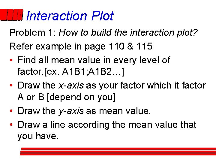
Interaction Plot Problem 1: How to build the interaction plot? Refer example in page 110 & 115 • Find all mean value in every level of factor. [ex. A 1 B 1; A 1 B 2…] • Draw the x-axis as your factor which it factor A or B [depend on you] • Draw the y-axis as mean value. • Draw a line according the mean value that you have.

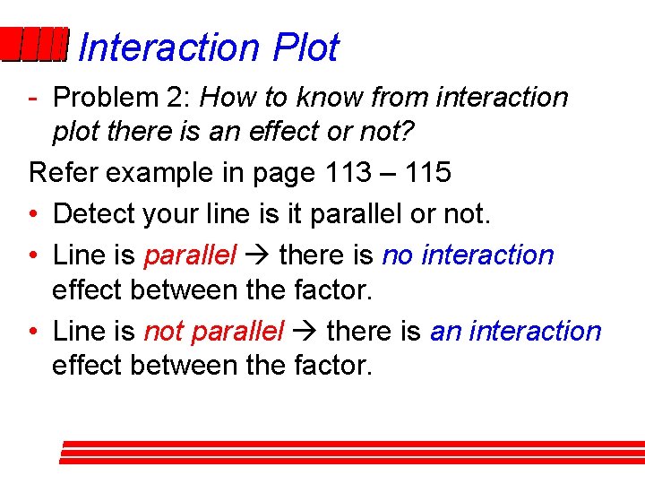
Interaction Plot - Problem 2: How to know from interaction plot there is an effect or not? Refer example in page 113 – 115 • Detect your line is it parallel or not. • Line is parallel there is no interaction effect between the factor. • Line is not parallel there is an interaction effect between the factor.

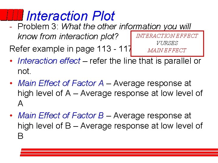
Interaction Plot - Problem 3: What the other information you will INTERACTION EFFECT know from interaction plot? VURSES Refer example in page 113 - 117 MAIN EFFECT • Interaction effect – refer the line that is parallel or not. • Main Effect of Factor A – Average response at high level of A – Average response at low level of A • Main Effect of Factor B – Average response at high level of B – Average response at low level of B

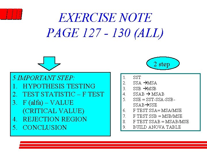
EXERCISE NOTE PAGE 127 - 130 (ALL) 2 step 5 IMPORTANT STEP: 1. HYPOTHESIS TESTING 2. TEST STATISTIC – F TEST 3. F (alfa) – VALUE (CRITICAL VALUE) 4. REJECTION REGION 5. CONCLUSION 1. 2. 3. 4. 5. 6. 7. 8. 9. SST SSA MSA SSB MSB SSAB MSAB SSE = SST-SSA-SSBSSAB SSE F TEST SSA= MSA/MSE F TEST SSB = MSB/MSE F TEST SSAB = MSAB/MSE BUILD ANOVA TABLE