CHAPTER 3 AGGREGATE PLANNING LEARNING OBJECTIVES l Define

CHAPTER 3 AGGREGATE PLANNING

LEARNING OBJECTIVES l Define aggregate planning and how it is useful l Identify optional strategies for developing an aggregate plan. l Prepare and solve an aggregate plan via graphical and quantitative method. l Understand Solve a yield management problem.

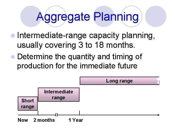
Aggregate Planning l Intermediate-range capacity planning, usually covering 3 to 18 months. l Determine the quantity and timing of production for the immediate future Long range Short range Now Intermediate range 2 months 1 Year

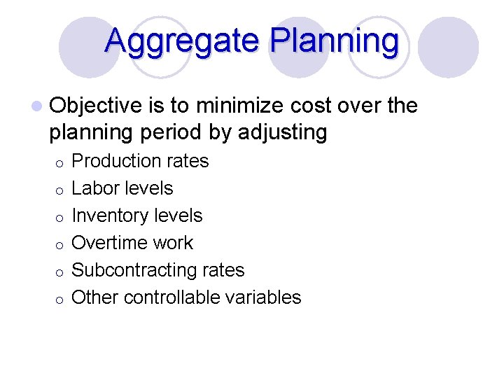
Aggregate Planning l Objective is to minimize cost over the planning period by adjusting ¡ ¡ ¡ Production rates Labor levels Inventory levels Overtime work Subcontracting rates Other controllable variables

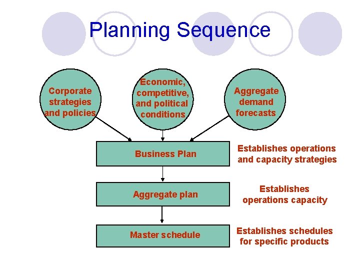
Planning Sequence Corporate strategies and policies Economic, competitive, and political conditions Business Plan Aggregate demand forecasts Establishes operations and capacity strategies Aggregate plan Establishes operations capacity Master schedule Establishes schedules for specific products

Aggregate Planning l Begin with forecast of aggregate demand l Forecast intermediate range l General plan to meet demand by setting ¡ ¡ ¡ Output levels Employment Finished goods inventory level l Production plan is the output of aggregate planning

Aggregate Planning Inputs l Resources ¡ Workforce ¡ Facilities l Demand forecast l Policies ¡ Subcontracting ¡ Overtime ¡ Inventory levels ¡ Back orders l Costs ¡ Inventory carrying ¡ Back orders ¡ Hiring/firing ¡ Overtime ¡ Inventory changes ¡ Subcontracting

Aggregate Planning Outputs l Total cost of a plan l Projected levels of inventory ¡ ¡ ¡ Inventory Output Employment Subcontracting Backordering

Aggregate Planning Strategies l Proactive ¡ Alter demand to match capacity l Reactive ¡ Alter capacity to match demand l Mixed ¡ Some of each

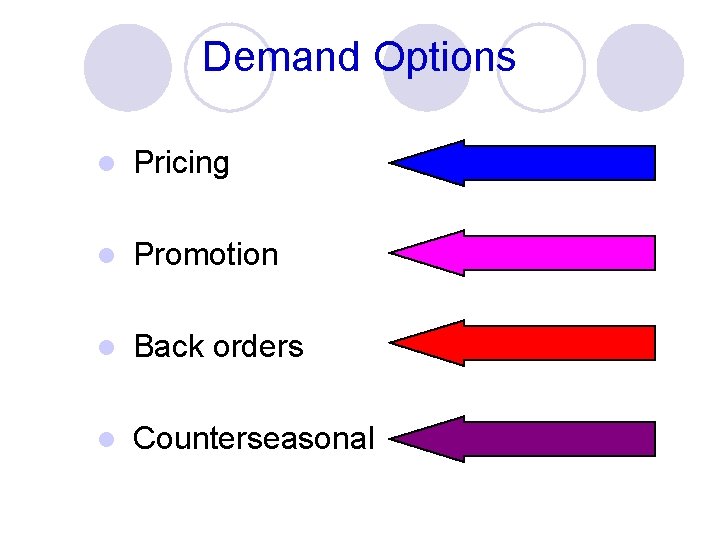
Demand Options l Pricing l Promotion l Back orders l Counterseasonal

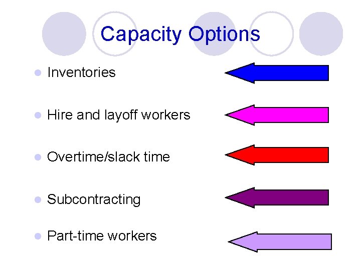
Capacity Options l Inventories l Hire and layoff workers l Overtime/slack time l Subcontracting l Part-time workers

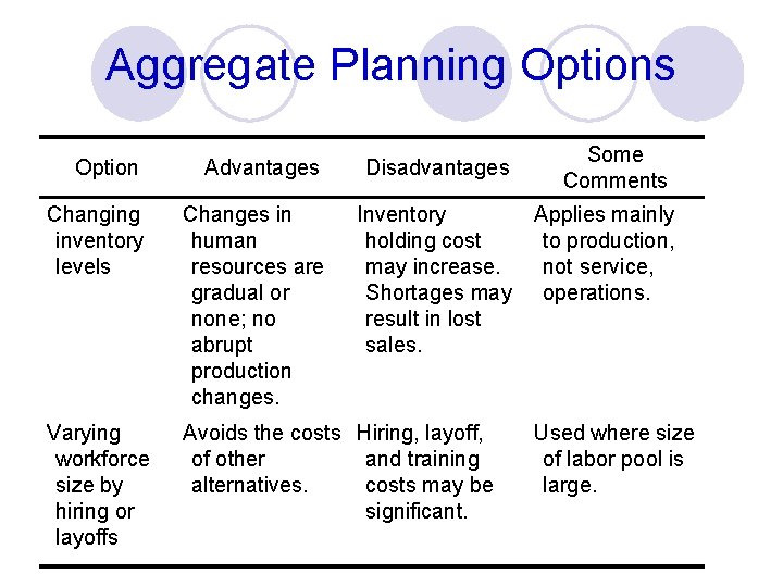
Aggregate Planning Options Option Advantages Disadvantages Changing inventory levels Changes in human resources are gradual or none; no abrupt production changes. Inventory holding cost may increase. Shortages may result in lost sales. Varying workforce size by hiring or layoffs Avoids the costs Hiring, layoff, of other and training alternatives. costs may be significant. Some Comments Applies mainly to production, not service, operations. Used where size of labor pool is large.

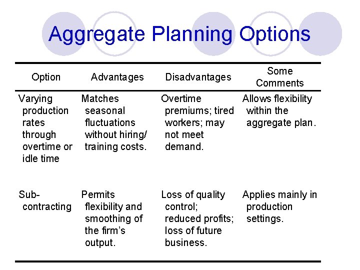
Aggregate Planning Options Option Advantages Disadvantages Some Comments Varying Matches production seasonal rates fluctuations through without hiring/ overtime or training costs. idle time Overtime Allows flexibility premiums; tired within the workers; may aggregate plan. not meet demand. Sub. Permits contracting flexibility and smoothing of the firm’s output. Loss of quality Applies mainly in control; production reduced profits; settings. loss of future business.

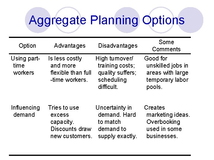
Aggregate Planning Options Option Advantages Disadvantages Some Comments Using parttime workers Is less costly High turnover/ and more training costs; flexible than full quality suffers; -time workers. scheduling difficult. Good for unskilled jobs in areas with large temporary labor pools. Influencing demand Tries to use Uncertainty in excess demand. Hard capacity. to match Discounts draw demand to new customers. supply exactly. Creates marketing ideas. Overbooking used in some businesses.

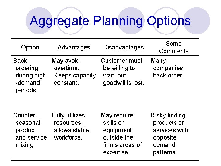
Aggregate Planning Options Option Advantages Disadvantages Some Comments Back May avoid Customer must ordering overtime. be willing to during high Keeps capacity wait, but -demand constant. goodwill is lost. periods Many companies back order. Counter. Fully utilizes seasonal resources; product allows stable and service workforce. mixing Risky finding products or services with opposite demand patterns. May require skills or equipment outside the firm’s areas of expertise.

Mixing Options l Chase ¡ Matching capacity to demand; the planned output for a period is set at the expected demand for that period l Level ¡ demand strategy: capacity strategy: Maintaining a steady rate of regular-time output while meeting variations in demand by a combination of options.

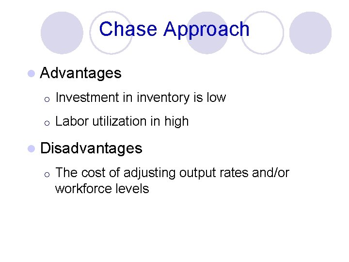
Chase Approach l Advantages ¡ Investment in inventory is low ¡ Labor utilization in high l Disadvantages ¡ The cost of adjusting output rates and/or workforce levels

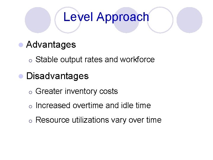
Level Approach l Advantages ¡ Stable output rates and workforce l Disadvantages ¡ Greater inventory costs ¡ Increased overtime and idle time ¡ Resource utilizations vary over time

Graphical Methods l Popular techniques l Easy to understand use l Trial-and-error approaches that do not guarantee an optimal solution l Require only limited computations

Techniques for Aggregate Planning 1. Determine demand for each period 2. Determine capacities for each period 3. Determine units costs 4. Identify policies that are pertinent 5. Develop alternative plans and costs 6. Select the best plan that satisfies objectives. Otherwise return to step 5.

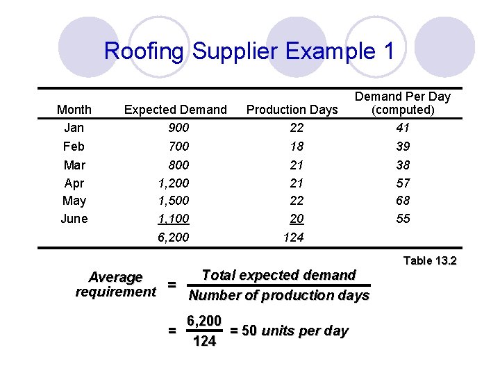
Roofing Supplier Example 1 Month Jan Expected Demand 900 Production Days 22 Feb Mar Apr May June 700 800 1, 200 1, 500 1, 100 18 21 21 22 20 6, 200 124 Demand Per Day (computed) 41 39 38 57 68 55 Table 13. 2 Total expected demand Average requirement = Number of production days = 6, 200 = 50 units per day 124

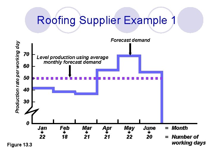
Production rate per working day Roofing Supplier Example 1 Forecast demand 70 – 60 – Level production using average monthly forecast demand 50 – 40 – 30 – Jan Feb Mar Apr May June 22 18 21 21 22 20 Figure 13. 3 = Month = Number of working days

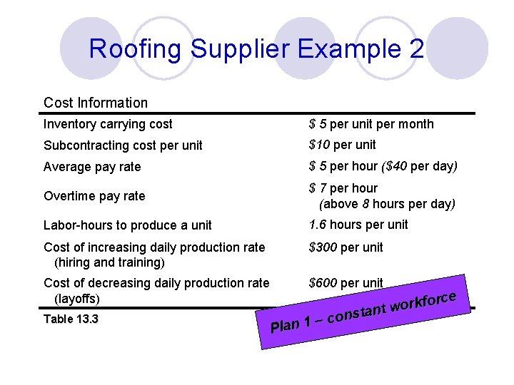
Roofing Supplier Example 2 Cost Information Inventory carrying cost $ 5 per unit per month Subcontracting cost per unit $10 per unit Average pay rate $ 5 per hour ($40 per day) Overtime pay rate $ 7 per hour (above 8 hours per day) Labor-hours to produce a unit 1. 6 hours per unit Cost of increasing daily production rate (hiring and training) $300 per unit Cost of decreasing daily production rate (layoffs) $600 per unit Table 13. 3 Plan rce o f k r o nt w a t s n o 1–c

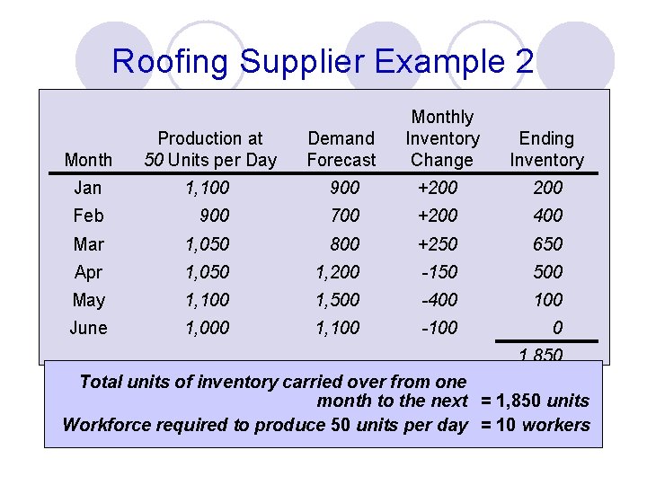
Roofing Supplier Example 2 Cost Information Production at Inventory Month carry 50 cost Units per Day Subcontracting cost per unit Jan 1, 100 Monthly Demand Inventory Ending per unit per month Forecast $ 5 Change Inventory 900 $10 +200 per unit 900 700 $ 5 per hour ($40 per 400 day) +200 Mar pay rate 1, 050 Overtime 800 $ 7 per hour +250 650 (above 8 hours per day) Average Feb pay rate Apr 1, 050 1, 200 May 1, 100 1, 500 Labor-hours to produce a unit Cost of increasing daily production rate June and training) 1, 000 1, 100 (hiring 200 -150 500 -400 100 -100 0 1. 6 hours per unit $300 per unit Cost of decreasing daily production rate $600 per unit 1, 850 (layoffs) Total units of inventory carried over from one t workforce tan ns monthnto the = 1, 850 units conext – 1 Pla Workforce required to produce 50 units per day = 10 workers Table 13. 3

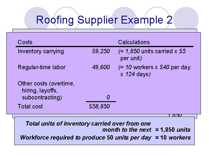
Roofing Supplier Example 2 Monthly Calculations Demand Inventory Ending $ 5 Change perunits unit per month Inventory carrying (= 1, 850 carried x $5 Month carry 50 cost Units per Day $9, 250 Forecast Inventory unit) $10 per unit Subcontracting cost per unit Jan 1, 100 900 per +200 Regular-time labor 900 49, 600 x $40 per day $ 5 workers per hour ($40 day) Average Feb pay rate 700 (= 10 +200 400 x 124 days) $ 7 per hour Mar pay rate 1, 050 800 +250 650 Overtime (above 8 hours per day) Other costs (overtime, Apr layoffs, 1, 050 1, 200 -150 500 hiring, 1. 6 hours per unit Labor-hours to produce a unit May 1, 100 1, 500 -400 100 subcontracting) 0 Costs. Information Production at Cost of increasing daily production rate Junecost 1, 000 1, 100 Total $58, 850 (hiring and training) $300 per unit -100 Cost of decreasing daily production rate $600 per unit (layoffs) Total units of inventory carried over from one 0 1, 850 month to the next = 1, 850 units Workforce required to produce 50 units per day = 10 workers Table 13. 3

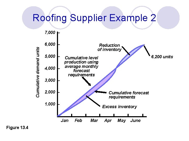
Roofing Supplier Example 2 Cumulative demand units 7, 000 – 6, 000 – 5, 000 – 4, 000 – Reduction of inventory 3, 000 – 2, 000 – Cumulative forecast requirements 1, 000 – – Figure 13. 4 6, 200 units Cumulative level production using average monthly forecast requirements Excess inventory Jan Feb Mar Apr May June

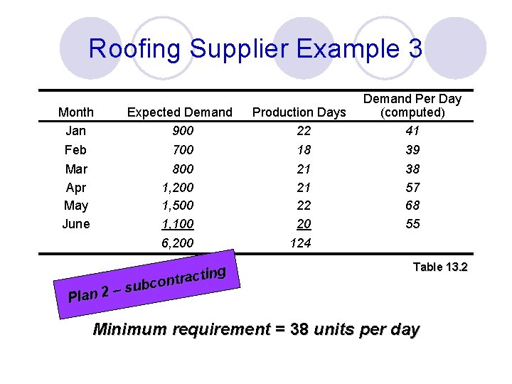
Roofing Supplier Example 3 Month Jan Expected Demand 900 Feb Mar Apr May June 700 800 1, 200 1, 500 1, 100 18 21 21 22 20 6, 200 124 Plan ting c a r t n co 2 – sub Production Days 22 Demand Per Day (computed) 41 39 38 57 68 55 Table 13. 2 Minimum requirement = 38 units per day

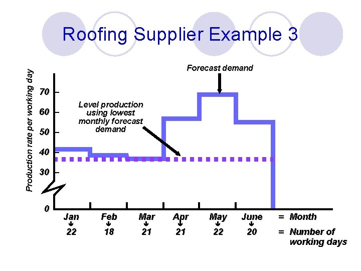
Production rate per working day Roofing Supplier Example 3 Forecast demand 70 – Level production using lowest monthly forecast demand 60 – 50 – 40 – 30 – Jan Feb Mar Apr May June 22 18 21 21 22 20 = Month = Number of working days

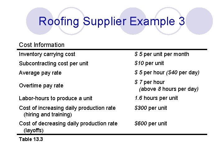
Roofing Supplier Example 3 Cost Information Inventory carrying cost $ 5 per unit per month Subcontracting cost per unit $10 per unit Average pay rate $ 5 per hour ($40 per day) Overtime pay rate $ 7 per hour (above 8 hours per day) Labor-hours to produce a unit 1. 6 hours per unit Cost of increasing daily production rate (hiring and training) $300 per unit Cost of decreasing daily production rate (layoffs) $600 per unit Table 13. 3

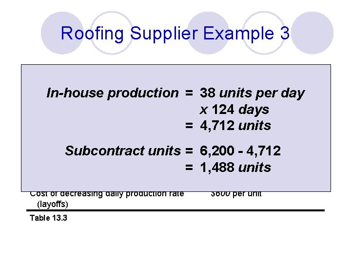
Roofing Supplier Example 3 Cost Information Inventory carry cost $ 5 per unit per month In-house production = 38$10 units per day per unit x $124 5 perdays hour ($40 per day) Average pay rate = 4, 712 $ 7 perunits hour Overtime pay rate Subcontracting cost per unit Subcontract Labor-hours to produce a unit (above 8 hours per day) units = 6, 200 - 4, 712 1. 6 hours per units Cost of increasing daily production rate = 1, 488 $300 per unit (hiring and training) Cost of decreasing daily production rate (layoffs) Table 13. 3 $600 per unit

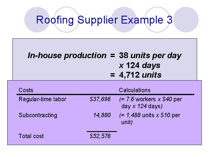
Roofing Supplier Example 3 Cost Information $ 5 per unit per month Inventory carry cost In-house production = 38$10 units per day per unit x $124 5 perdays hour ($40 per day) Average pay rate = 4, 712 $ 7 perunits hour Overtime pay rate Subcontracting cost per unit (above 8 hours per day) Costs Subcontract Labor-hours to produce a units = Calculations 6, 200 - 4, 712 1. 6 hours per unit Regular-time labor $37, 696 7. 6 workers 1, 488 units Cost of increasing daily production rate = (= $300 per unit x $40 per day x 124 days) (hiring and training) Cost of decreasing daily production rate Subcontracting 14, 880 (layoffs) Table 13. 3 Total cost $52, 576 unitx $10 per (= $600 1, 488 per units unit)

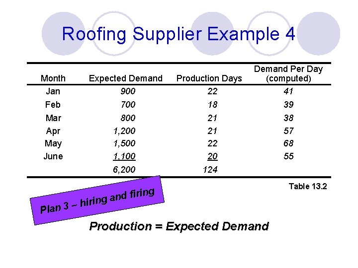
Roofing Supplier Example 4 Month Jan Expected Demand 900 Production Days 22 Feb Mar Apr May June 700 800 1, 200 1, 500 1, 100 18 21 21 22 20 6, 200 124 Demand Per Day (computed) 41 firing d n a iring h – 3 Plan Production = Expected Demand 39 38 57 68 55 Table 13. 2

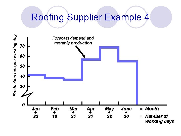
Production rate per working day Roofing Supplier Example 4 Forecast demand monthly production 70 – 60 – 50 – 40 – 30 – Jan Feb Mar Apr May June 22 18 21 21 22 20 = Month = Number of working days

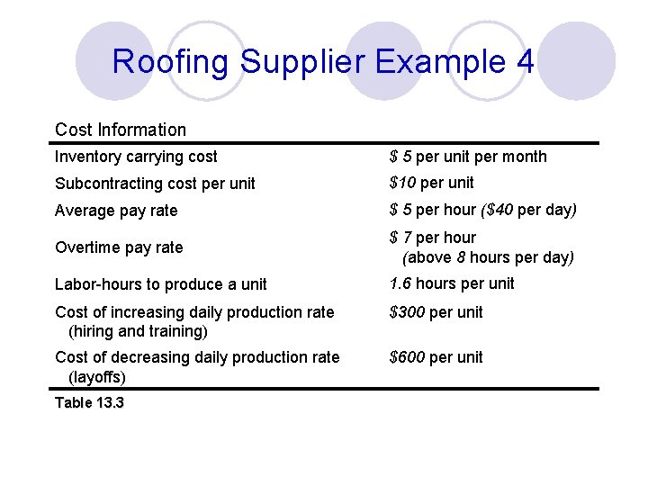
Roofing Supplier Example 4 Cost Information Inventory carrying cost $ 5 per unit per month Subcontracting cost per unit $10 per unit Average pay rate $ 5 per hour ($40 per day) Overtime pay rate $ 7 per hour (above 8 hours per day) Labor-hours to produce a unit 1. 6 hours per unit Cost of increasing daily production rate (hiring and training) $300 per unit Cost of decreasing daily production rate (layoffs) $600 per unit Table 13. 3

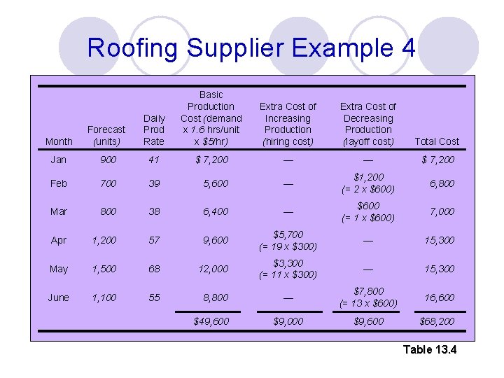
Roofing Supplier Example 4 Cost Information Inventory carrying. Daily cost Forecast Month (units) Subcontracting Prod Rate cost per Jan 900 Average pay rate Basic Production Cost (demand x 1. 6 hrs/unitx $5/hr) Extra Cost of Increasing $ 5 per Decreasing unit per month Production (hiring cost) Total Cost $10 per(layoff unit cost) 41 $ 7, 200 — — ($40 per $day) 7, 200 $ 5 per hour 6, 800 $ 7 per(=hour 2 x $600) (above 8$600 hours per day) Feb 700 39 5, 600 — Mar 800 38 6, 400 — Overtime pay rate Labor-hours to produce a unit Apr Cost 1, 200 57 increasing daily of (hiring and training) May 1, 500 68 9, 600 production 12, 000 $49, 600 1. 6 (= 1 per x $600) hours unit $5, 700 rate(= 19 x $300) $300 — per unit $3, 300 rate(= 11 x $300) $600 per unit Cost of decreasing daily production (layoffs) June 1, 100 55 8, 800 Table 13. 3 $1, 200 7, 000 15, 300 — $7, 800 (= 13 x $600) 16, 600 $9, 000 $9, 600 $68, 200 Table 13. 4

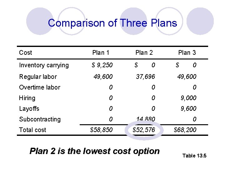
Comparison of Three Plans Cost Plan 1 Plan 2 Inventory carrying $ 9, 250 $ Regular labor 49, 600 37, 696 49, 600 Overtime labor 0 0 0 Hiring 0 0 9, 000 Layoffs 0 0 9, 600 Subcontracting 0 14, 880 0 $58, 850 $52, 576 $68, 200 Total cost 0 Plan 2 is the lowest cost option Plan 3 $ 0 Table 13. 5

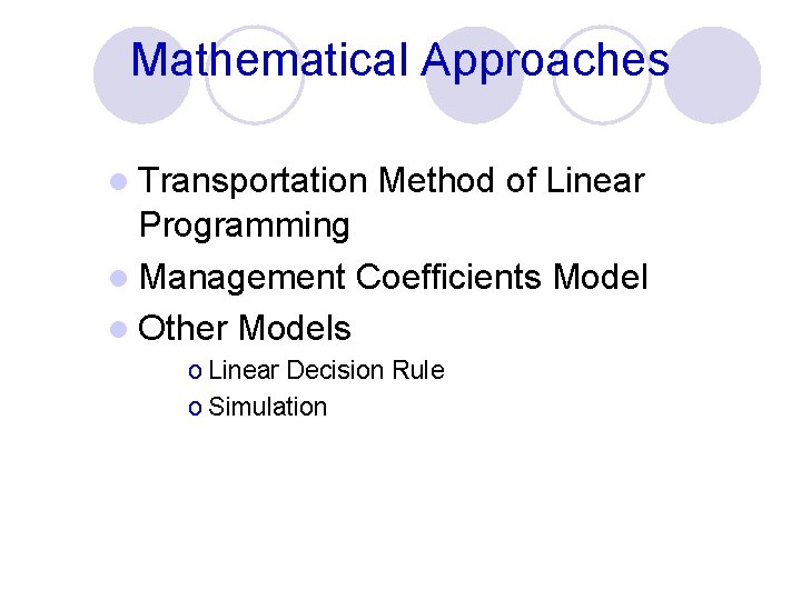
Mathematical Approaches l Transportation Method of Linear Programming l Management Coefficients Model l Other Models o Linear Decision Rule o Simulation

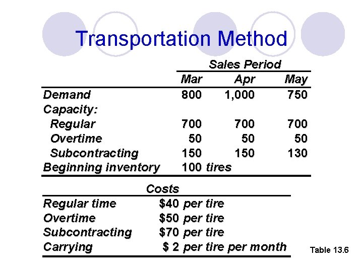
Transportation Method Demand Capacity: Regular Overtime Subcontracting Beginning inventory Regular time Overtime Subcontracting Carrying Sales Period Mar Apr May 800 1, 000 750 700 50 50 150 100 tires Costs $40 per tire $50 per tire $70 per tire $ 2 per tire per month 700 50 130 Table 13. 6

Transportation Example Important points 1. Carrying costs are $2/tire/month. If goods are made in one period and held over to the next, holding costs are incurred 2. Supply must equal demand, so a dummy column called “unused capacity” is added 3. Because back ordering is not viable in this example, cells that might be used to satisfy earlier demand are not available

Transportation Example Important points 4. Quantities in each column designate the levels of inventory needed to meet demand requirements 5. In general, production should be allocated to the lowest cost cell available without exceeding unused capacity in the row or demand in the column

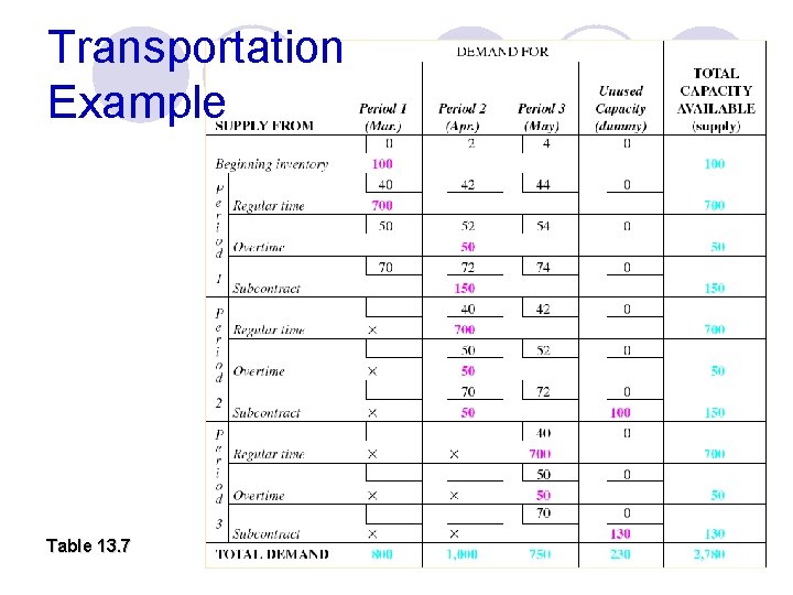
Transportation Example Table 13. 7

Yield Management Allocating company scarce resources to customers at prices that will maximize yield or revenue. l Charging different prices l Discount l

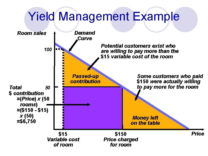
Yield Management Example Demand Curve Room sales Potential customers exist who are willing to pay more than the $15 variable cost of the room 100 Passed-up contribution 50 Total $ contribution =(Price) x (50 rooms) =($150 - $15) x (50) =$6, 750 $15 Variable cost of room Some customers who paid $150 were actually willing to pay more for the room Money left on the table $150 Price charged for room Price

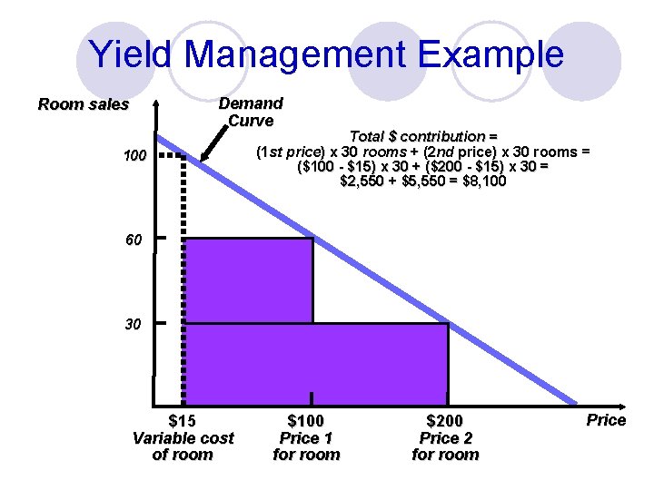
Yield Management Example Demand Curve Room sales 100 Total $ contribution = (1 st price) x 30 rooms + (2 nd price) x 30 rooms = ($100 - $15) x 30 + ($200 - $15) x 30 = $2, 550 + $5, 550 = $8, 100 60 30 $15 Variable cost of room $100 Price 1 for room $200 Price 2 for room Price

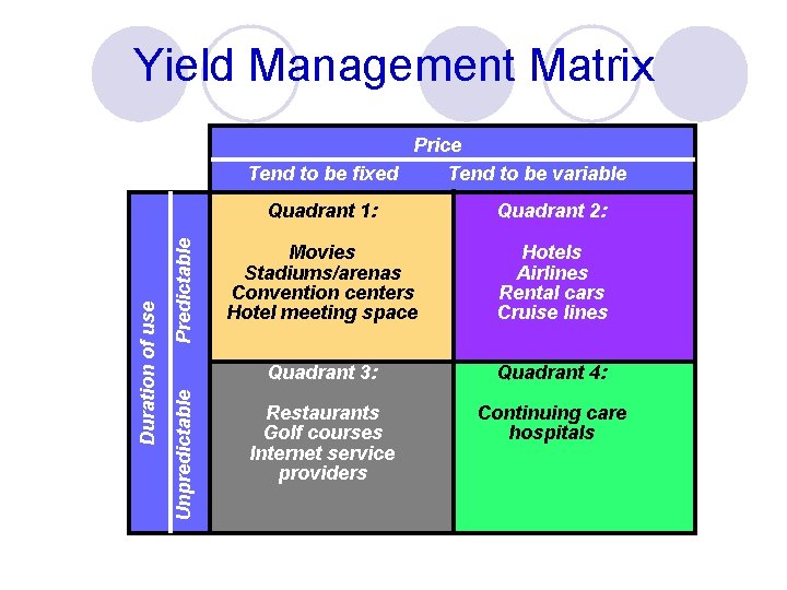
Yield Management Matrix Predictable Unpredictable Duration of use Price Tend to be fixed Tend to be variable Quadrant 1: Quadrant 2: Movies Stadiums/arenas Convention centers Hotel meeting space Hotels Airlines Rental cars Cruise lines Quadrant 3: Quadrant 4: Restaurants Golf courses Internet service providers Continuing care hospitals

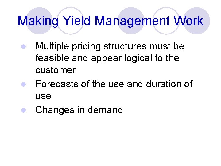
Making Yield Management Work Multiple pricing structures must be feasible and appear logical to the customer l Forecasts of the use and duration of use l Changes in demand l