Chapter 27 Linear Filtering Part I Kalman Filter

Chapter 27: Linear Filtering - Part I: Kalman Filter Standard Kalman filtering – Linear dynamics

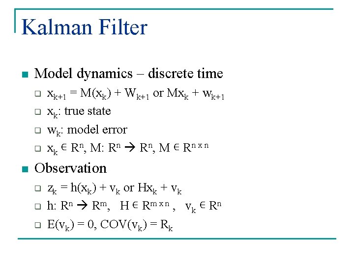
Kalman Filter n Model dynamics – discrete time q q n xk+1 = M(xk) + Wk+1 or Mxk + wk+1 xk: true state wk: model error xk ∊ Rn, M: Rn Rn, M ∊ Rn x n Observation q q q zk = h(xk) + vk or Hxk + vk h: Rn Rm, H ∊ Rm x n , vk ∊ Rn E(vk) = 0, COV(vk) = Rk

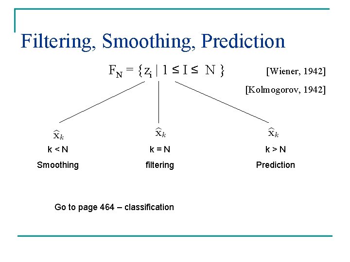
Filtering, Smoothing, Prediction FN = {zi | 1 ≤ I ≤ N } [Wiener, 1942] [Kolmogorov, 1942] k<N k=N k>N Smoothing filtering Prediction Go to page 464 – classification

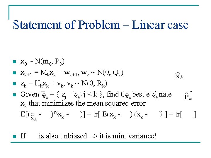
Statement of Problem – Linear case n n n x 0 ~ N(m 0, P 0) xk+1 = Mkxk + wk+1, wk ~ N(0, Qk) zk = Hkxk + vk, vk ~ N(0, Rk) Given Fk = { zj | 1 ≤ j ≤ k }, find the best estimate of xk that minimizes the mean squared error E[(xk - )T(xk )] = tr[ E(xk - )T] = tr[ ] If is also unbiased => it is min. variance!

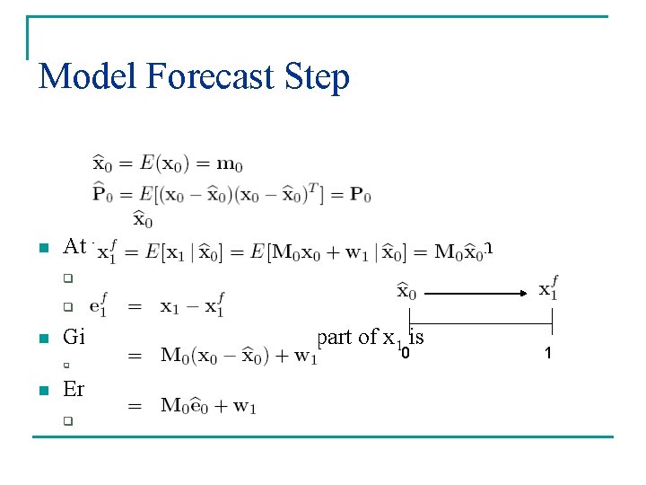
Model Forecast Step n At time k = 0, F 0 – initial information is given q q n Given , the predictable part of x 1 is q n Error in prediction q 0 1

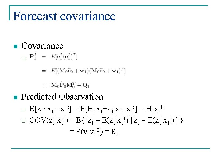
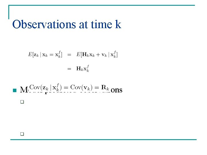
Forecast covariance n Covariance q n Predicted Observation q q E[z 1/ x 1= x 1 f] = E[H 1 x 1+v 1|x 1=x 1 f] = H 1 x 1 f COV(z 1|x 1 f) = E{[z 1 – E(z 1|x 1 f)]T} = E(v 1 v 1 T) = R 1

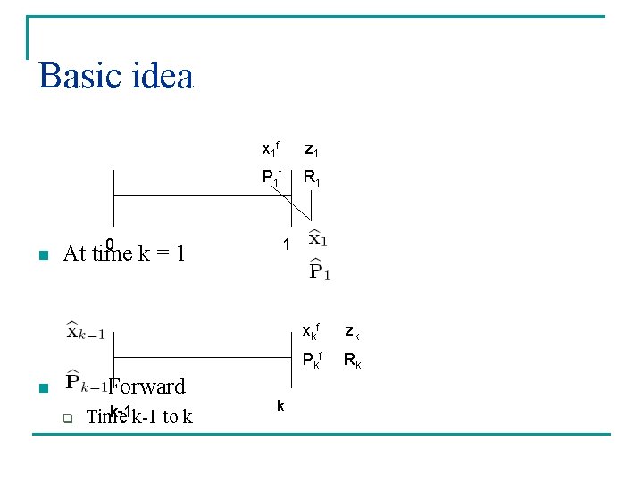
Basic idea n n 0 At time k=1 Fast Forward q k-1 k-1 to k Time x 1 f z 1 P 1 f R 1 1 k xkf zk Pk f Rk

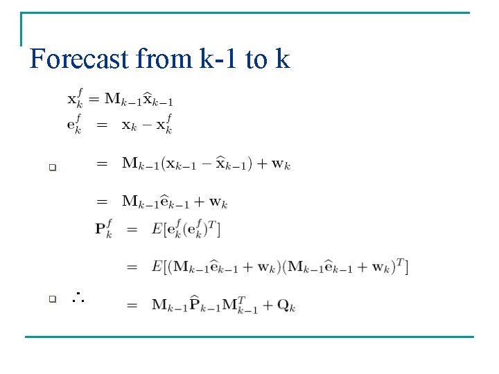
Forecast from k-1 to k q q ∴

Observations at time k n Model predicted observations q q

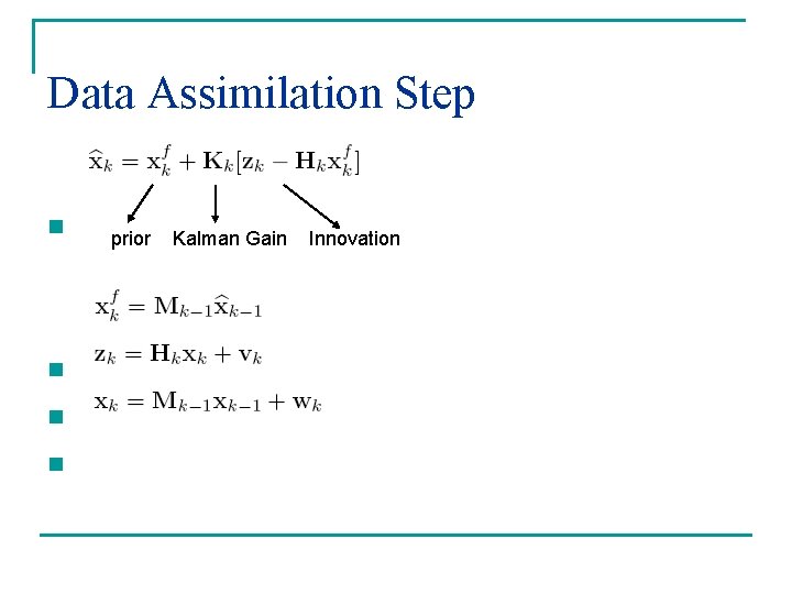
Data Assimilation Step n n prior Kalman Gain Innovation

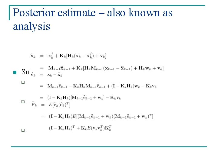
Posterior estimate – also known as analysis n Substitute and simplify q q q

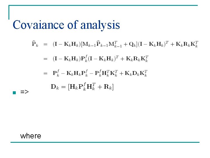
Covaiance of analysis n => where

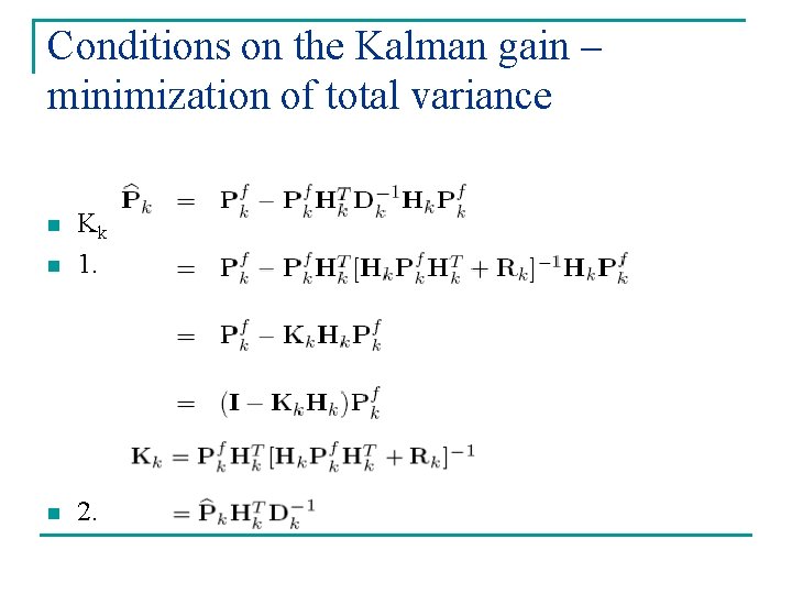
Conditions on the Kalman gain – minimization of total variance n Kk = Pkf. Hk. TDk-1 = Pkf. Hk. T[Hk. Pkf. Hk. T + Rk]-1 1. n 2. n

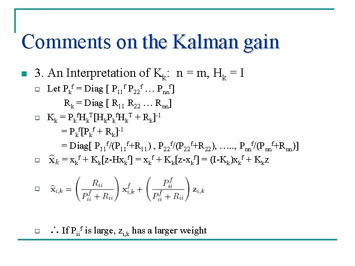
Comments on the Kalman gain n 3. An Interpretation of Kk: n = m, Hk = I q q q Let Pkf = Diag [ P 11 f P 22 f … Pnnf] Rk = Diag [ R 11 R 22 … Rnn] Kk = Pkf. Hk. T[Hk. Pkf. Hk. T + Rk]-1 = Pkf[Pkf + Rk]-1 = Diag[ P 11 f/(P 11 f+R 11) , P 22 f/(P 22 f+R 22), …. . , Pnnf/(Pnnf+Rnn)] = xkf + Kk[z-Hxkf] = xkf + Kk[z-xkf] = (I-Kk)xkf + Kkz q q ∴ If Piif is large, zi, k has a larger weight

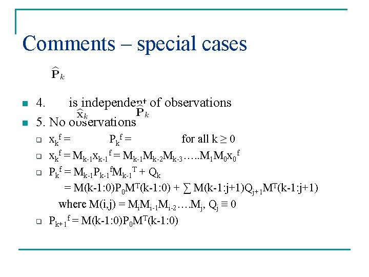
Comments – special cases n n 4. is independent of observations 5. No observations q q xkf = Pkf = for all k ≥ 0 xkf = Mk-1 xk-1 f = Mk-1 Mk-2 Mk-3…. . M 1 M 0 x 0 f Pkf = Mk-1 Pk-1 f. Mk-1 T + Qk = M(k-1: 0)P 0 MT(k-1: 0) + ∑ M(k-1: j+1)Qj+1 MT(k-1: j+1) where M(i, j) = Mi. Mi-1 Mi-2…. Mj, Qj ≡ 0 Pk+1 f = M(k-1: 0)P 0 MT(k-1: 0)

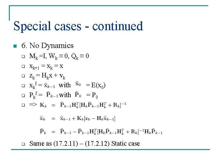
Special cases - continued n 6. No Dynamics q Mk =I, Wk ≡ 0, Qk ≡ 0 xk+1 = xk = x zk = Hkx + vk xkf = with = E(x 0) P kf = with = P 0 => q Same as (17. 2. 11) – (17. 2. 12) Static case q q q

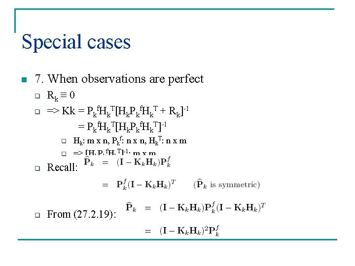
Special cases n 7. When observations are perfect q q Rk ≡ 0 => Kk = Pkf. Hk. T[Hk. Pkf. Hk. T + Rk]-1 = Pkf. Hk. T[Hk. Pkf. Hk. T]-1 q q Hk: m x n, Pkf: n x n, Hk. T: n x m => [Hk. Pkf. Hk. T]-1: m x m q Recall: q From (27. 2. 19):

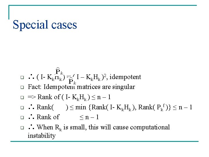
Special cases q q q ∴ ( I- Kk. Hk ) = ( I – Kk. Hk )2, idempotent Fact: Idempotent matrices are singular => Rank of ( I- Kk. Hk ) ≤ n – 1 ∴ Rank( ) ≤ min {Rank( I- Kk. Hk ), Rank( Pkf )} ≤ n – 1 ∴ Rank of ≤n– 1 ∴ When Rk is small, this will cause computational instability

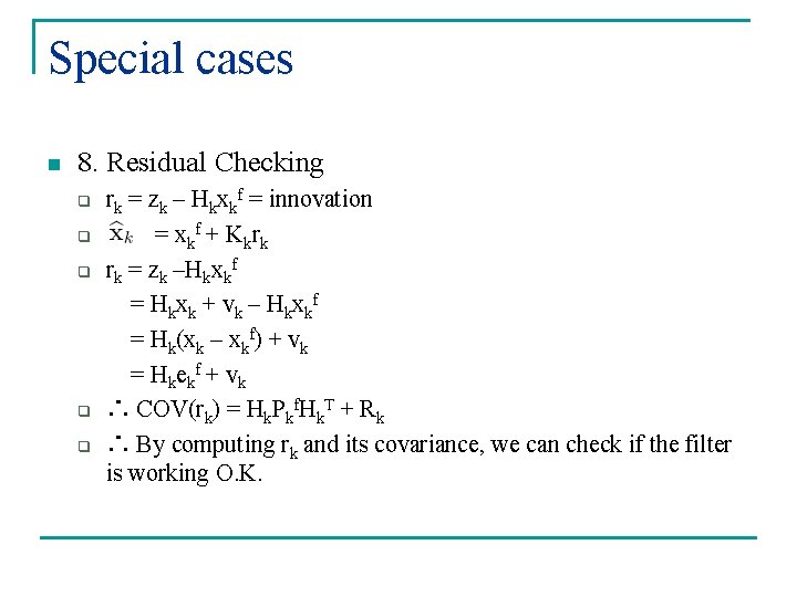
Special cases n 8. Residual Checking q q q rk = zk – Hkxkf = innovation = xkf + Kkrk rk = zk –Hkxkf = Hkxk + vk – Hkxkf = Hk(xk – xkf) + vk = Hkekf + vk ∴ COV(rk) = Hk. Pkf. Hk. T + Rk ∴ By computing rk and its covariance, we can check if the filter is working O. K.

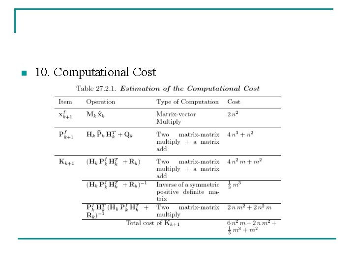
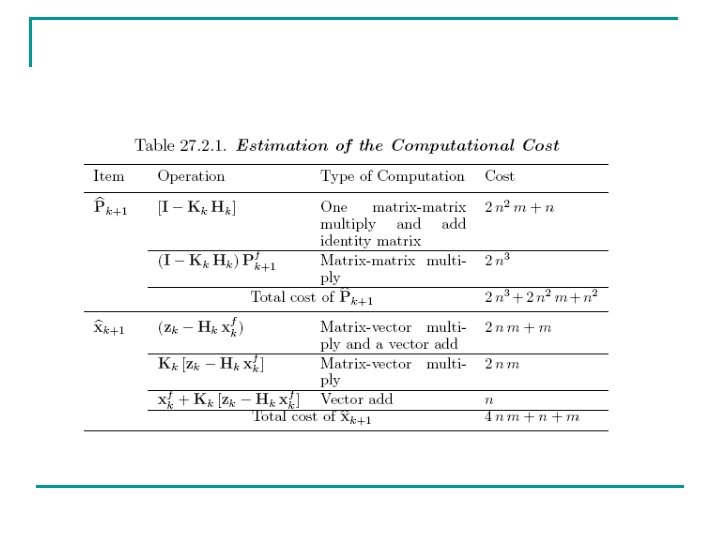
n 10. Computational Cost

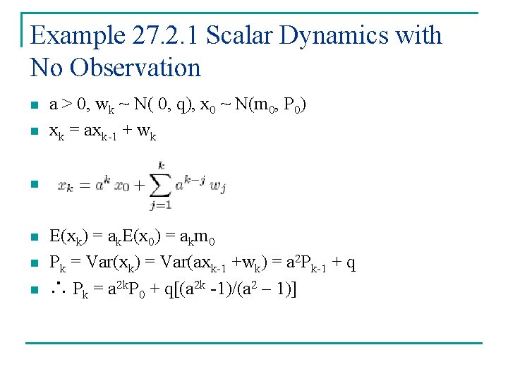
Example 27. 2. 1 Scalar Dynamics with No Observation n n a > 0, wk ~ N( 0, q), x 0 ~ N(m 0, P 0) xk = axk-1 + wk n n E(xk) = ak. E(x 0) = akm 0 Pk = Var(xk) = Var(axk-1 +wk) = a 2 Pk-1 + q ∴ Pk = a 2 k. P 0 + q[(a 2 k -1)/(a 2 – 1)]

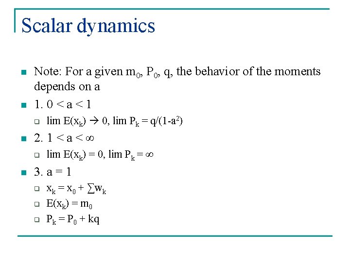
Scalar dynamics n n Note: For a given m 0, P 0, q, the behavior of the moments depends on a 1. 0 < a < 1 q n 2. 1 < a < ∞ q n lim E(xk) 0, lim Pk = q/(1 -a 2) lim E(xk) = 0, lim Pk = ∞ 3. a = 1 q q q xk = x 0 + ∑wk E(xk) = m 0 Pk = P 0 + kq

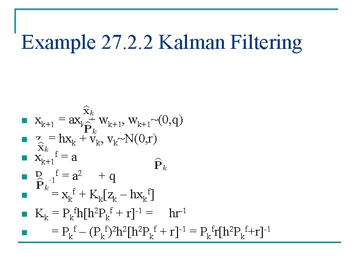
Example 27. 2. 2 Kalman Filtering n n n n xk+1 = axk + wk+1, wk+1~(0, q) zk = hxk + vk, vk~N(0, r) xk+1 f = a Pk+1 f = a 2 + q = xkf + Kk[zk – hxkf] Kk = Pkfh[h 2 Pkf + r]-1 = hr-1 = Pkf – (Pkf)2 h 2[h 2 Pkf + r]-1 = Pkfr[h 2 Pkf+r]-1

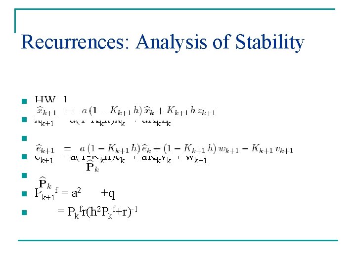
Recurrences: Analysis of Stability n n HW. 1 xk+1 f = a(1 -Kkh)xkf + a. Kkzk n n ek+1 f = a(1 -Kkh)ekf + a. Kkvk + wk+1 n n n Pk+1 f = a 2 +q = Pkfr(h 2 Pkf+r)-1

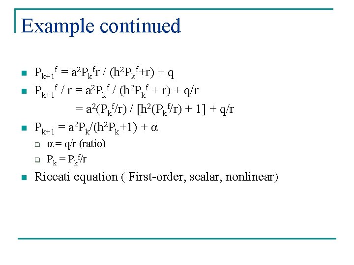
Example continued n n n Pk+1 f = a 2 Pkfr / (h 2 Pkf+r) + q Pk+1 f / r = a 2 Pkf / (h 2 Pkf + r) + q/r = a 2(Pkf/r) / [h 2(Pkf/r) + 1] + q/r Pk+1 = a 2 Pk/(h 2 Pk+1) + α q q n α = q/r (ratio) Pk = Pkf/r Riccati equation ( First-order, scalar, nonlinear)

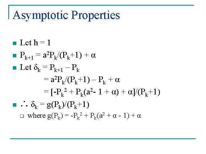
Asymptotic Properties n n Let h = 1 Pk+1 = a 2 Pk/(Pk+1) + α Let δk = Pk+1 – Pk = a 2 Pk/(Pk+1) – Pk + α = [-Pk 2 + Pk(a 2 - 1 + α) + α]/(Pk+1) ∴ δk = g(Pk)/(Pk+1) q where g(Pk) = -Pk 2 + Pk(a 2 + α - 1) + α

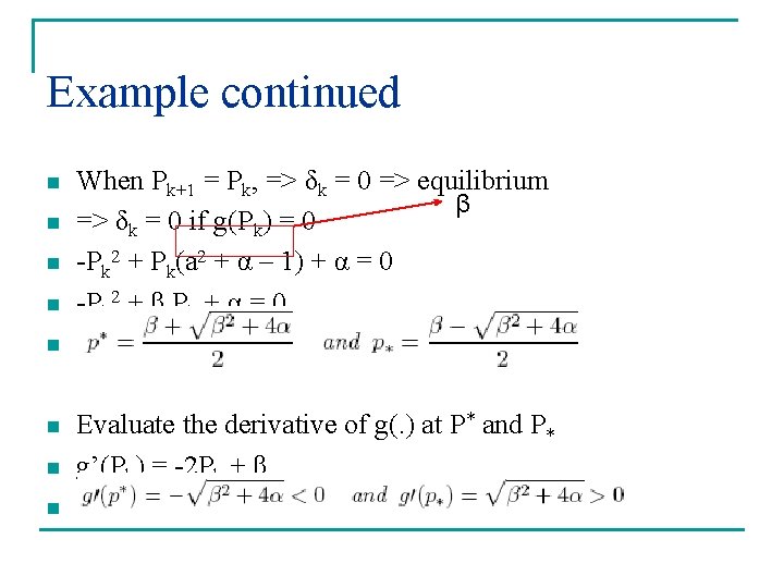
Example continued n n When Pk+1 = Pk, => δk = 0 => equilibrium β => δk = 0 if g(Pk) = 0 -Pk 2 + Pk(a 2 + α – 1) + α = 0 -Pk 2 + β Pk + α = 0 n n Evaluate the derivative of g(. ) at P* and P* g’(Pk) = -2 Pk + β

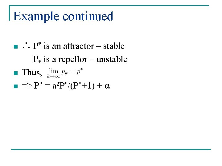
Example continued n n n ∴ P* is an attractor – stable P* is a repellor – unstable Thus, => P* = a 2 P*/(P*+1) + α

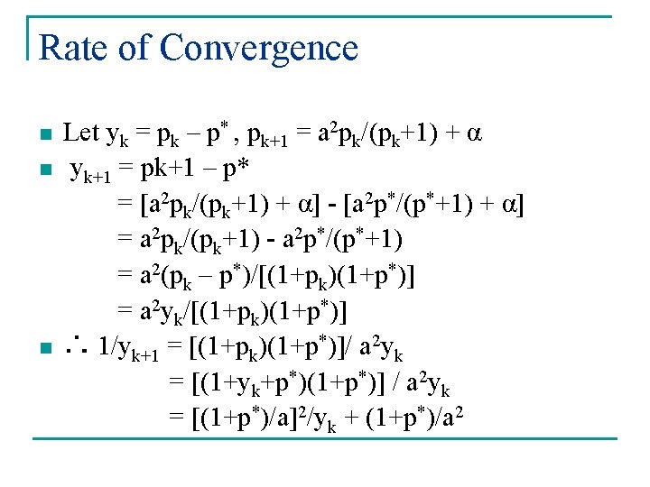
Rate of Convergence n n n Let yk = pk – p* , pk+1 = a 2 pk/(pk+1) + α yk+1 = pk+1 – p* = [a 2 pk/(pk+1) + α] - [a 2 p*/(p*+1) + α] = a 2 pk/(pk+1) - a 2 p*/(p*+1) = a 2(pk – p*)/[(1+pk)(1+p*)] = a 2 yk/[(1+pk)(1+p*)] ∴ 1/yk+1 = [(1+pk)(1+p*)]/ a 2 yk = [(1+yk+p*)(1+p*)] / a 2 yk = [(1+p*)/a]2/yk + (1+p*)/a 2

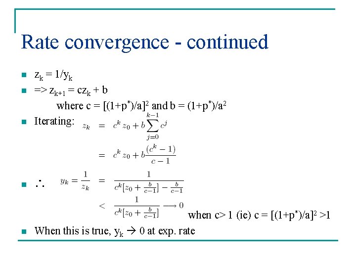
Rate convergence - continued n zk = 1/yk => zk+1 = czk + b where c = [(1+p*)/a]2 and b = (1+p*)/a 2 Iterating: n ∴ n when c> 1 (ie) c = [(1+p*)/a]2 >1 When this is true, yk 0 at exp. rate n n

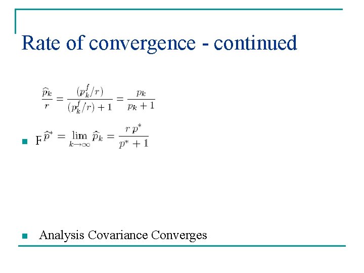
Rate of convergence - continued n n From (27. 2. 38) h = 1 Analysis Covariance Converges

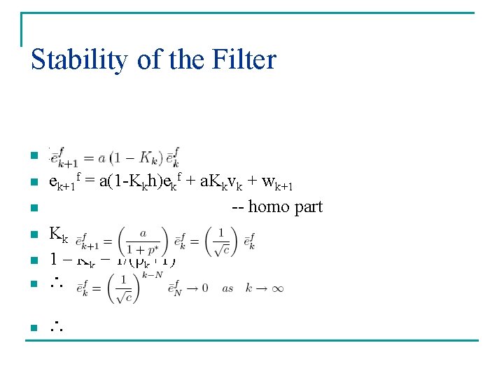
Stability of the Filter n h=1 ek+1 f = a(1 -Kkh)ekf + a. Kkvk + wk+1 -- homo part Kk = pkf/(pkf+r) = pk/(pk+1) 1 – Kk = 1/(pk+1) n ∴ n n