Chapter 26 Inferences for Regression Copyright 2015 2010

Chapter 26 Inferences for Regression Copyright © 2015, 2010, 2007 Pearson Education, Inc. Chapter 26, Slide 1 -1 1

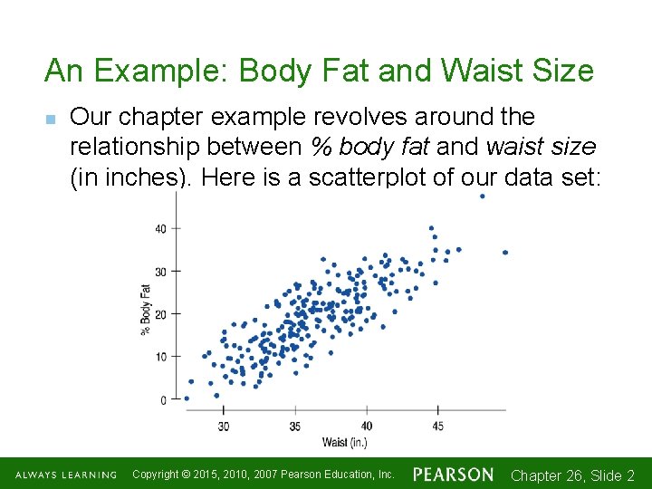
An Example: Body Fat and Waist Size n Our chapter example revolves around the relationship between % body fat and waist size (in inches). Here is a scatterplot of our data set: Copyright © 2015, 2010, 2007 Pearson Education, Inc. Chapter 26, Slide 1 -2 2

Remembering Regression n n In regression, we want to model the relationship between two quantitative variables, one the predictor and the other the response. To do that, we imagine an idealized regression line, which assumes that the means of the distributions of the response variable fall along the line even though individual values are scattered around it. Copyright © 2015, 2010, 2007 Pearson Education, Inc. Chapter 26, Slide 1 -3 3

Remembering Regression (cont. ) n n Now we’d like to know what the regression model can tell us beyond the individuals in the study. We want to make confidence intervals and test hypotheses about the slope and intercept of the regression line. Copyright © 2015, 2010, 2007 Pearson Education, Inc. Chapter 26, Slide 1 -4 4

The Population and the Sample n n n When we found a confidence interval for a mean, we could imagine a single, true underlying value for the mean. When we tested whether two means or two proportions were equal, we imagined a true underlying difference. What does it mean to do inference for regression? Copyright © 2015, 2010, 2007 Pearson Education, Inc. Chapter 26, Slide 1 -5 5

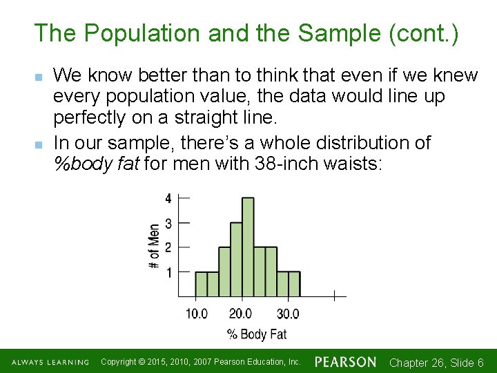
The Population and the Sample (cont. ) n n We know better than to think that even if we knew every population value, the data would line up perfectly on a straight line. In our sample, there’s a whole distribution of %body fat for men with 38 -inch waists: Copyright © 2015, 2010, 2007 Pearson Education, Inc. Chapter 26, Slide 1 -6 6

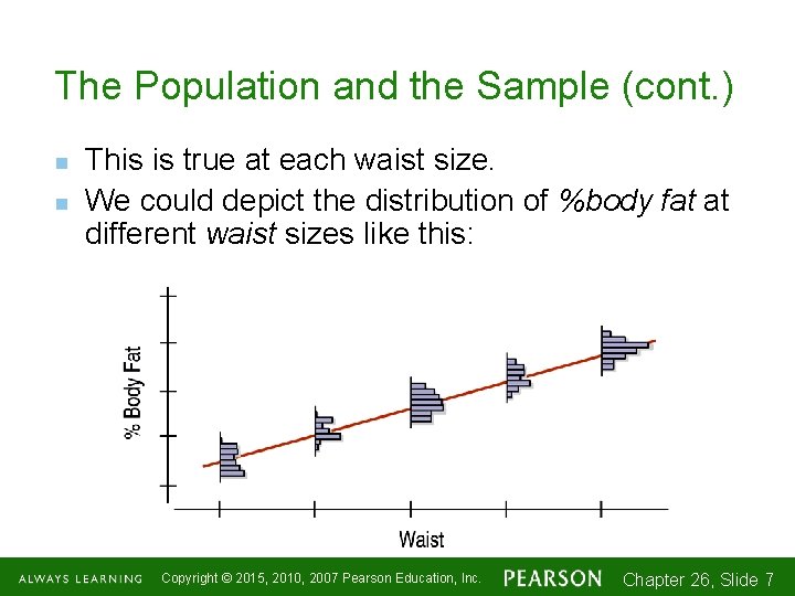
The Population and the Sample (cont. ) n n This is true at each waist size. We could depict the distribution of %body fat at different waist sizes like this: Copyright © 2015, 2010, 2007 Pearson Education, Inc. Chapter 26, Slide 1 -7 7

The Population and the Sample (cont. ) n n n The model assumes that the means of the distributions of %body fat for each waist size fall along the line even though the individuals are scattered around it. The model is not a perfect description of how the variables are associated, but it may be useful. If we had all the values in the population, we could find the slope and intercept of the idealized regression line explicitly by using least squares. Copyright © 2015, 2010, 2007 Pearson Education, Inc. Chapter 26, Slide 1 -8 8

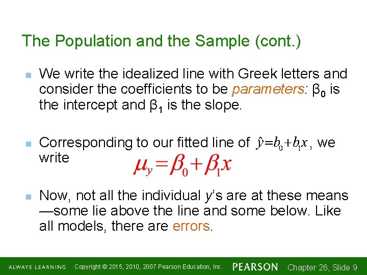
The Population and the Sample (cont. ) n n n We write the idealized line with Greek letters and consider the coefficients to be parameters: β 0 is the intercept and β 1 is the slope. Corresponding to our fitted line of write , we Now, not all the individual y’s are at these means —some lie above the line and some below. Like all models, there are errors. Copyright © 2015, 2010, 2007 Pearson Education, Inc. Chapter 26, Slide 1 -9 9

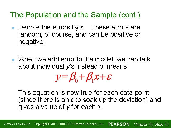
The Population and the Sample (cont. ) n n Denote the errors by ε. These errors are random, of course, and can be positive or negative. When we add error to the model, we can talk about individual y’s instead of means: This equation is now true for each data point (since there is an ε to soak up the deviation) and gives a value of y for each x. Copyright © 2015, 2010, 2007 Pearson Education, Inc. Chapter 26, Slide 1 -10 10

Assumptions and Conditions n n n In Chapter 7 when we fit lines to data, we needed to check only the Straight Enough Condition. Now, when we want to make inferences about the coefficients of the line, we’ll have to make more assumptions (and thus check more conditions). We need to be careful about the order in which we check conditions. If an initial assumption is not true, it makes no sense to check the later ones. Copyright © 2015, 2010, 2007 Pearson Education, Inc. Chapter 26, Slide 1 -11 11

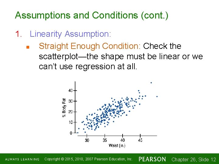
Assumptions and Conditions (cont. ) 1. Linearity Assumption: n Straight Enough Condition: Check the scatterplot—the shape must be linear or we can’t use regression at all. Copyright © 2015, 2010, 2007 Pearson Education, Inc. Chapter 26, Slide 1 -12 12

Assumptions and Conditions (cont. ) 1. Linearity Assumption: n If the scatterplot is straight enough, we can go on to some assumptions about the errors. If not, stop here, or consider re-expressing the data to make the scatterplot more nearly linear. n Check the Quantitative Data Condition. The data must be quantitative for this to make sense. Copyright © 2015, 2010, 2007 Pearson Education, Inc. Chapter 26, Slide 1 -13 13

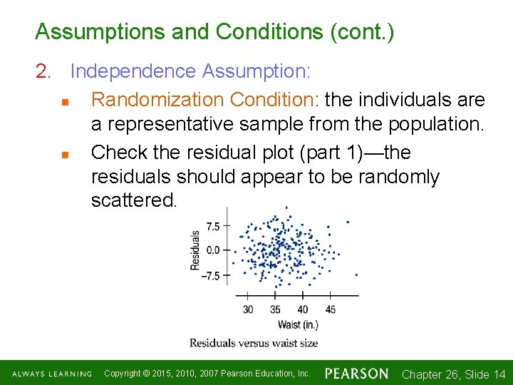
Assumptions and Conditions (cont. ) 2. Independence Assumption: n Randomization Condition: the individuals are a representative sample from the population. n Check the residual plot (part 1)—the residuals should appear to be randomly scattered. Copyright © 2015, 2010, 2007 Pearson Education, Inc. Chapter 26, Slide 1 -14 14

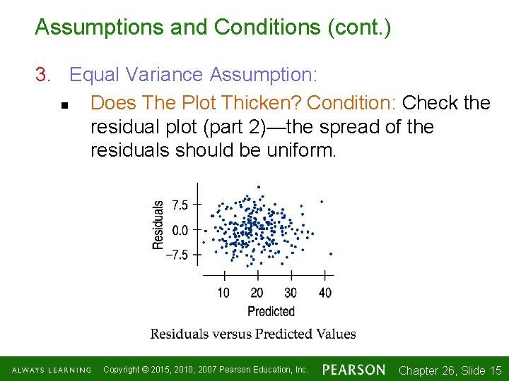
Assumptions and Conditions (cont. ) 3. Equal Variance Assumption: n Does The Plot Thicken? Condition: Check the residual plot (part 2)—the spread of the residuals should be uniform. Copyright © 2015, 2010, 2007 Pearson Education, Inc. Chapter 26, Slide 1 -15 15

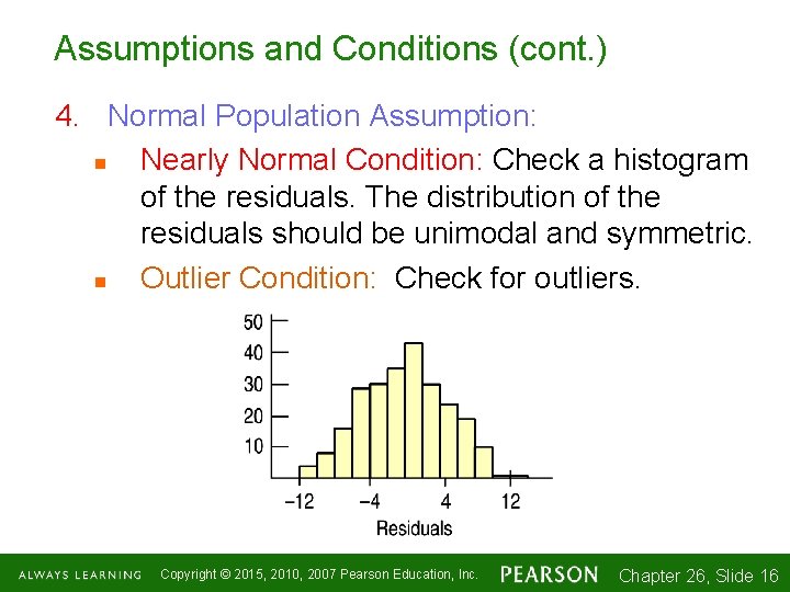
Assumptions and Conditions (cont. ) 4. Normal Population Assumption: n Nearly Normal Condition: Check a histogram of the residuals. The distribution of the residuals should be unimodal and symmetric. n Outlier Condition: Check for outliers. Copyright © 2015, 2010, 2007 Pearson Education, Inc. Chapter 26, Slide 1 -16 16

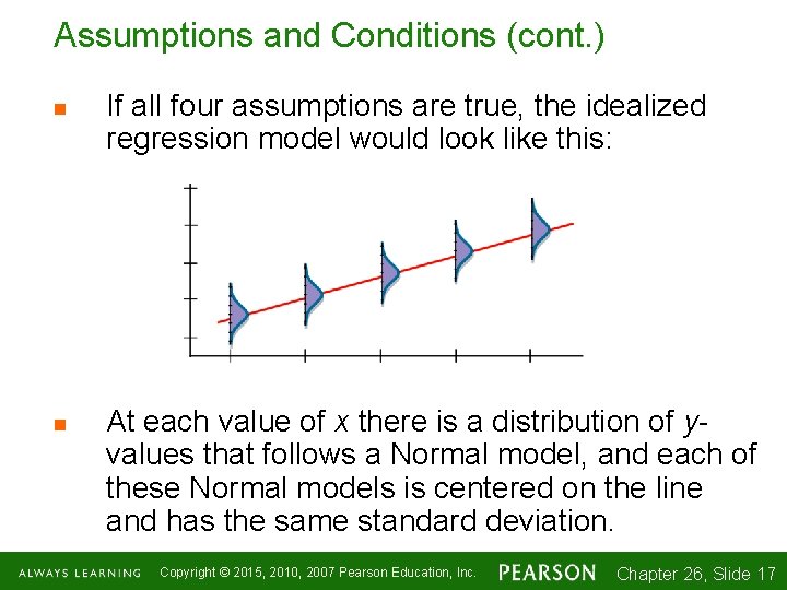
Assumptions and Conditions (cont. ) n n If all four assumptions are true, the idealized regression model would look like this: At each value of x there is a distribution of yvalues that follows a Normal model, and each of these Normal models is centered on the line and has the same standard deviation. Copyright © 2015, 2010, 2007 Pearson Education, Inc. Chapter 26, Slide 1 -17 17

Which Come First: the Conditions or the Residuals? n n n There’s a catch in regression—the best way to check many of the conditions is with the residuals, but we get the residuals only after we compute the regression model. To compute the regression model, however, we should check the conditions. So we work in this order: n Make a scatterplot of the data to check the Straight Enough Condition. (If the relationship isn’t straight, try re-expressing the data. Or stop. ) Copyright © 2015, 2010, 2007 Pearson Education, Inc. Chapter 26, Slide 1 -18 18

Which Come First: the Conditions or the Residuals? (cont. ) n n n If the data are straight enough, fit a regression model and find the residuals, e, and predicted values, . Make a scatterplot of the residuals against x or the predicted values. n This plot should have no pattern. Check in particular for any bend, any thickening (or thinning), or any outliers. If the data are measured over time, plot the residuals against time to check for evidence of patterns that might suggest they are not independent. Copyright © 2015, 2010, 2007 Pearson Education, Inc. Chapter 26, Slide 1 -19 19

Which Come First: the Conditions or the Residuals? (cont. ) n n If the scatterplots look OK, then make a histogram and Normal probability plot of the residuals to check the Nearly Normal Condition. If all the conditions seem to be satisfied, go ahead with inference. Copyright © 2015, 2010, 2007 Pearson Education, Inc. Chapter 26, Slide 1 -20 20

Intuition About Regression Inference n n n We expect any sample to produce a b 1 whose expected value is the true slope, β 1. What about its standard deviation? What aspects of the data affect how much the slope and intercept vary from sample to sample? Copyright © 2015, 2010, 2007 Pearson Education, Inc. Chapter 26, Slide 1 -21 21

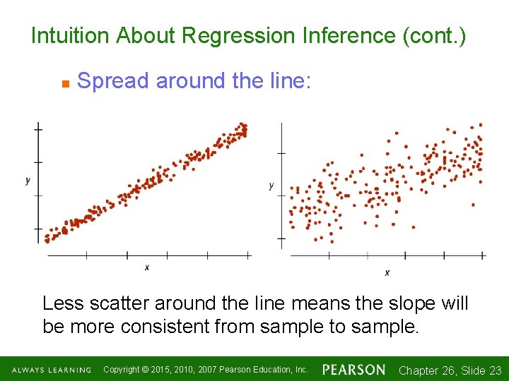
Intuition About Regression Inference (cont. ) n Spread around the line: Less scatter around the line means the slope will be more consistent from sample to sample. n The spread around the line is measured with the residual standard deviation se. n You can always find se in the regression output, often just labeled s. n Copyright © 2015, 2010, 2007 Pearson Education, Inc. Chapter 26, Slide 1 -22 22

Intuition About Regression Inference (cont. ) n Spread around the line: Less scatter around the line means the slope will be more consistent from sample to sample. Copyright © 2015, 2010, 2007 Pearson Education, Inc. Chapter 26, Slide 1 -23 23

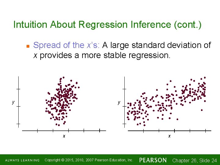
Intuition About Regression Inference (cont. ) n Spread of the x’s: A large standard deviation of x provides a more stable regression. Copyright © 2015, 2010, 2007 Pearson Education, Inc. Chapter 26, Slide 1 -24 24

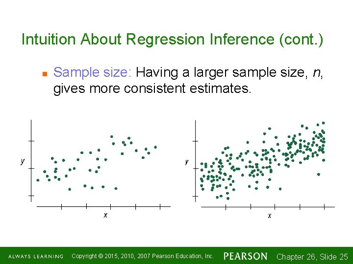
Intuition About Regression Inference (cont. ) n Sample size: Having a larger sample size, n, gives more consistent estimates. Copyright © 2015, 2010, 2007 Pearson Education, Inc. Chapter 26, Slide 1 -25 25

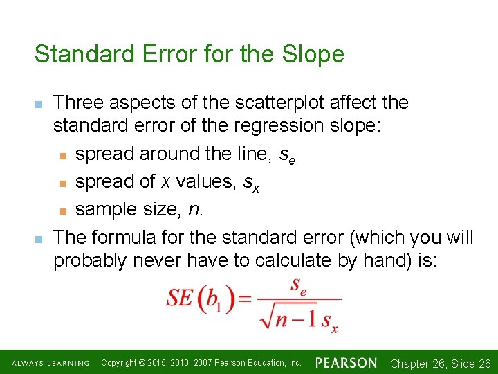
Standard Error for the Slope n n Three aspects of the scatterplot affect the standard error of the regression slope: n spread around the line, se n spread of x values, sx n sample size, n. The formula for the standard error (which you will probably never have to calculate by hand) is: Copyright © 2015, 2010, 2007 Pearson Education, Inc. Chapter 26, Slide 1 -26 26

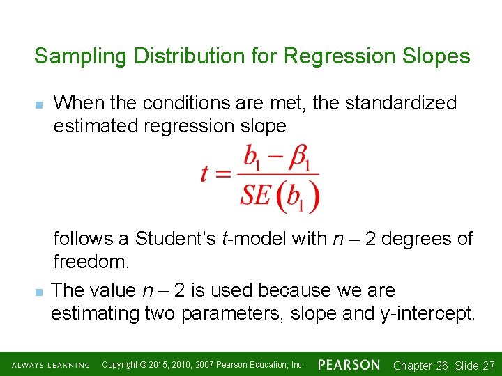
Sampling Distribution for Regression Slopes n n When the conditions are met, the standardized estimated regression slope follows a Student’s t-model with n – 2 degrees of freedom. The value n – 2 is used because we are estimating two parameters, slope and y-intercept. Copyright © 2015, 2010, 2007 Pearson Education, Inc. Chapter 26, Slide 1 -27 27

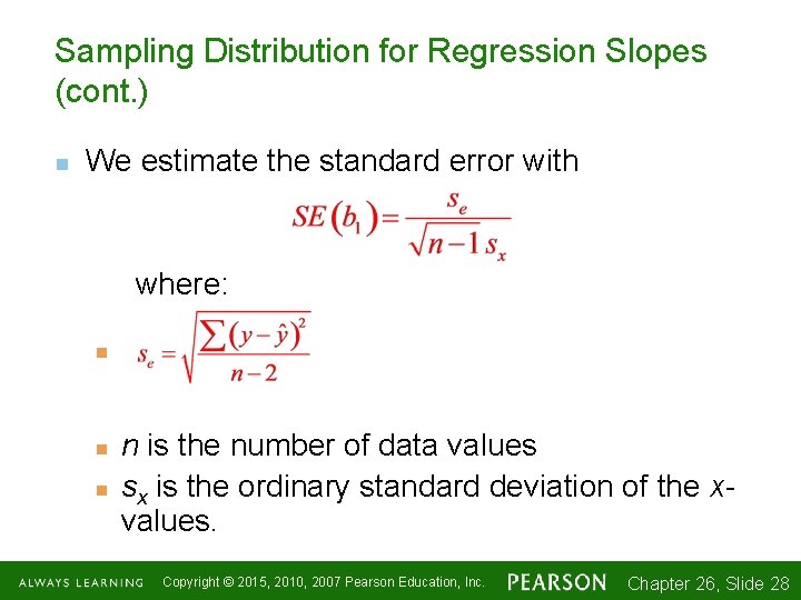
Sampling Distribution for Regression Slopes (cont. ) n We estimate the standard error with where: n n is the number of data values sx is the ordinary standard deviation of the xvalues. Copyright © 2015, 2010, 2007 Pearson Education, Inc. Chapter 26, Slide 1 -28 28

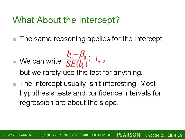
What About the Intercept? n The same reasoning applies for the intercept. n We can write but we rarely use this fact for anything. n The intercept usually isn’t interesting. Most hypothesis tests and confidence intervals for regression are about the slope. Copyright © 2015, 2010, 2007 Pearson Education, Inc. Chapter 26, Slide 1 -29 29

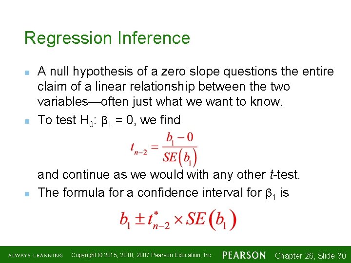
Regression Inference n A null hypothesis of a zero slope questions the entire claim of a linear relationship between the two variables—often just what we want to know. To test H 0: β 1 = 0, we find n and continue as we would with any other t-test. The formula for a confidence interval for β 1 is n Copyright © 2015, 2010, 2007 Pearson Education, Inc. Chapter 26, Slide 1 -30 30

What Can Go Wrong? n n n Don’t fit a linear regression to data that aren’t straight. Watch out for the plot thickening. n If the spread in y changes with x, our predictions will be very good for some x-values and very bad for others. Make sure the errors are Normal. n Check the histogram and Normal probability plot of the residuals to see if this assumption looks reasonable. Copyright © 2015, 2010, 2007 Pearson Education, Inc. Chapter 26, Slide 1 -31 31

What Can Go Wrong? (cont. ) n n n Watch out for extrapolation. n It’s always dangerous to predict for x-values that lie far from the center of the data. Watch out for high-influence points and outliers. Watch out for one-tailed tests. n Tests of hypotheses about regression coefficients are usually two-tailed, so software packages report two-tailed P-values. n If you are using software to conduct a onetailed test about slope, you’ll need to divide the reported P-value in half. Copyright © 2015, 2010, 2007 Pearson Education, Inc. Chapter 26, Slide 1 -32 32

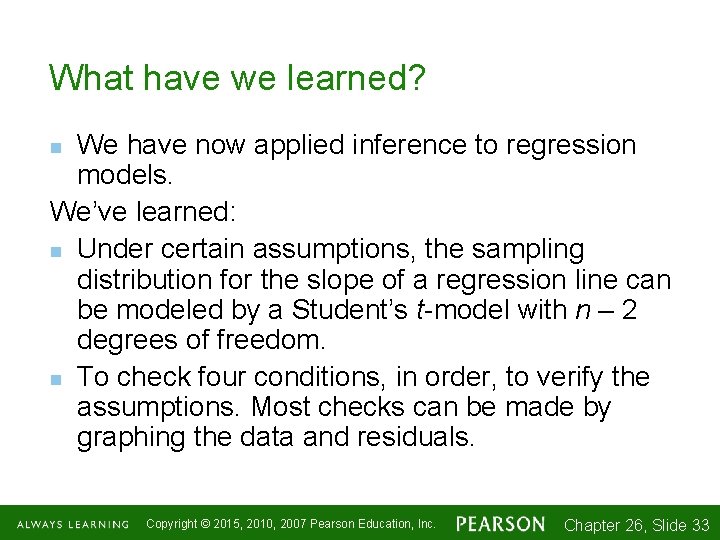
What have we learned? We have now applied inference to regression models. We’ve learned: n Under certain assumptions, the sampling distribution for the slope of a regression line can be modeled by a Student’s t-model with n – 2 degrees of freedom. n To check four conditions, in order, to verify the assumptions. Most checks can be made by graphing the data and residuals. n Copyright © 2015, 2010, 2007 Pearson Education, Inc. Chapter 26, Slide 1 -33 33

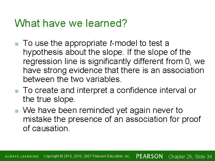
What have we learned? n n n To use the appropriate t-model to test a hypothesis about the slope. If the slope of the regression line is significantly different from 0, we have strong evidence that there is an association between the two variables. To create and interpret a confidence interval or the true slope. We have been reminded yet again never to mistake the presence of an association for proof of causation. Copyright © 2015, 2010, 2007 Pearson Education, Inc. Chapter 26, Slide 1 -34 34

AP Tips n n Often the AP test, for these procedures, will say “the conditions for inference have been satisfied”. Make sure to acknowledge this gift in your answer! Make sure you can read the regression output from a computer. This is how the AP test usually provides regression information. Copyright © 2015, 2010, 2007 Pearson Education, Inc. Chapter 26, Slide 1 -35 35

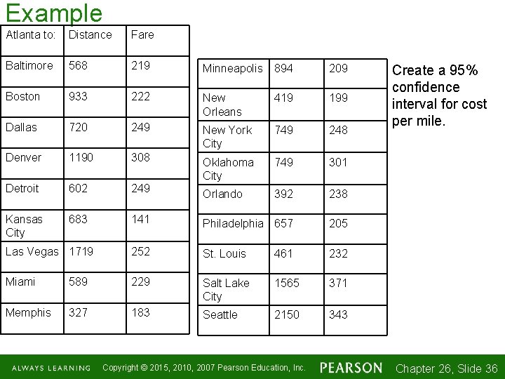
Example Atlanta to: Distance Fare Baltimore 568 219 Minneapolis 894 209 Boston 933 222 New Orleans 419 199 Dallas 720 249 New York City 749 248 Denver 1190 308 Oklahoma City 749 301 Detroit 602 249 Orlando 392 238 Kansas City 683 141 Philadelphia 657 205 Las Vegas 1719 252 St. Louis 461 232 Miami 589 229 Salt Lake City 1565 371 Memphis 327 183 Seattle 2150 343 Copyright © 2015, 2010, 2007 Pearson Education, Inc. Create a 95% confidence interval for cost per mile. Chapter 26, Slide 1 -36 36

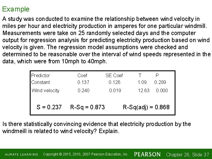
Example A study was conducted to examine the relationship between wind velocity in miles per hour and electricity production in amperes for one particular windmill. Measurements were take on 25 randomly selected days and the computer output for regression analysis for predicting electricity production based on wind velocity is given. The regression model assumptions were checked and determined to be reasonable over the interval of wind speeds represented in the data, which were from 10 mph to 40 mph. Predictor Constant Coef 0. 137 SE Coef 0. 126 Wind velocity 0. 240 0. 019 S = 0. 237 R-Sq = 0. 873 T 1. 09 12. 63 P 0. 289 0. 000 R-Sq(adj) = 0. 868 Is there statistically convincing evidence that electricity production by the windmeill is related to wind velocity? Explain. Copyright © 2015, 2010, 2007 Pearson Education, Inc. Chapter 26, Slide 1 -37 37