Chapter 26 Data Mining Some slides courtesy of

Chapter 26: Data Mining (Some slides courtesy of Rich Caruana, Cornell University)

Definition Data mining is the exploration and analysis of large quantities of data in order to discover valid, novel, potentially useful, and ultimately understandable patterns in data. Example pattern (Census Bureau Data): If (relationship = husband), then (gender = male). 99. 6%

Definition (Cont. ) Data mining is the exploration and analysis of large quantities of data in order to discover valid, novel, potentially useful, and ultimately understandable patterns in data. Valid: The patterns hold in general. Novel: We did not know the pattern beforehand. Useful: We can devise actions from the patterns. Understandable: We can interpret and comprehend the patterns.

Why Use Data Mining Today? Human analysis skills are inadequate: • Volume and dimensionality of the data • High data growth rate Availability of: • • • Data Storage Computational power Off-the-shelf software Expertise

An Abundance of Data • • • Supermarket scanners, POS data Preferred customer cards Credit card transactions Direct mail response Call center records ATM machines Demographic data Sensor networks Cameras Web server logs Customer web site trails

Commercial Support • Many data mining tools • http: //www. kdnuggets. com/software • Database systems with data mining support • Visualization tools • Data mining process support • Consultants

Why Use Data Mining Today? Competitive pressure! “The secret of success is to know something that nobody else knows. ” Aristotle Onassis • Competition on service, not only on price (Banks, phone companies, hotel chains, rental car companies) • Personalization • CRM • The real-time enterprise • Security, homeland defense

Types of Data • Relational data and transactional data • Spatial and temporal data, spatio-temporal observations • Time-series data • Text • Voice • Images, video • Mixtures of data • Sequence data • Features from processing other data sources

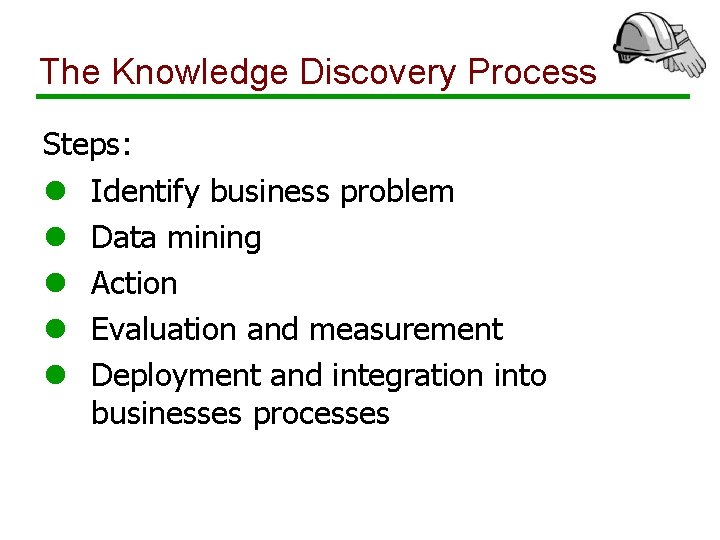
The Knowledge Discovery Process Steps: l Identify business problem l Data mining l Action l Evaluation and measurement l Deployment and integration into businesses processes

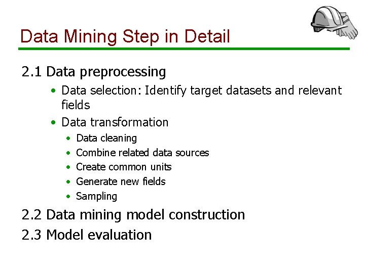
Data Mining Step in Detail 2. 1 Data preprocessing • Data selection: Identify target datasets and relevant fields • Data transformation • • • Data cleaning Combine related data sources Create common units Generate new fields Sampling 2. 2 Data mining model construction 2. 3 Model evaluation

Data Selection • Data Sources are Expensive • Obtaining Data • Loading Data into Database • Maintaining Data • Most Fields are not useful • Names • Addresses • Code Numbers Ramakrishnan and Gehrke. Database Management Systems, 3 rd Edition.

Data Cleaning • Missing Data • Unknown demographic data • Impute missing values when possible • Incorrect Data • Hand-typed default values (e. g. 1900 for dates) • Misplaced Fields • Data does not always match documentation • Missing Relationships • Foreign keys missing or dangling Ramakrishnan and Gehrke. Database Management Systems, 3 rd Edition.

Combining Data Sources • Enterprise Data typically stored in many heterogeneous systems • Keys to join systems may or may not be present • Heuristics must be used when keys are missing • Time-based matching • Situation-based matching Ramakrishnan and Gehrke. Database Management Systems, 3 rd Edition.

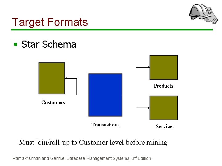
Create Common Units • Data exists at different Granularity Levels • Customers • Transactions • Products • Data Mining requires a common Granularity Level (often called a Case) • Mining usually occurs at “customer” or similar granularity Ramakrishnan and Gehrke. Database Management Systems, 3 rd Edition.

Generate New Fields • Raw data fields may not be useful by themselves • Simple transformations can improve mining results dramatically: • Customer start date Customer tenure • Recency, Frequency, Monetary values • Fields at wrong granularity level must be aggregated Ramakrishnan and Gehrke. Database Management Systems, 3 rd Edition.

Sampling • Most real datasets are too large to mine directly (> 200 million cases) • Apply random sampling to reduce data size and improve error estimation • Always sample at analysis granularity (case/”customer”), never at transaction granularity. Ramakrishnan and Gehrke. Database Management Systems, 3 rd Edition.

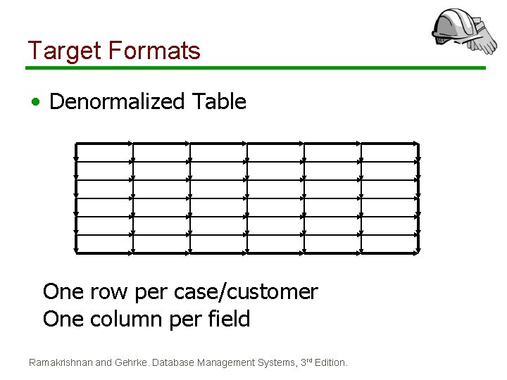
Target Formats • Denormalized Table One row per case/customer One column per field Ramakrishnan and Gehrke. Database Management Systems, 3 rd Edition.

Target Formats • Star Schema Products Customers Transactions Services Must join/roll-up to Customer level before mining Ramakrishnan and Gehrke. Database Management Systems, 3 rd Edition.

Data Transformation Example • Client: major health insurer • Business Problem: determine when the web is effective at deflecting call volume • Data Sources • • Call center records Web data Claims Customer and Provider database Ramakrishnan and Gehrke. Database Management Systems, 3 rd Edition.

Data Transformation Example • Cleaning Required • • • Dirty reason codes in call center records Missing customer Ids in some web records No session information in web records Incorrect date fields in claims Missing values in customer and provider records • Some customer records missing entirely Ramakrishnan and Gehrke. Database Management Systems, 3 rd Edition.

Data Transformation Example • Combining Data Sources • Systems use different keys. Mappings were provided, but not all rows joined properly. • Web data difficult to match due to missing customer Ids on certain rows. • Call center rows incorrectly combined portions of different calls. Ramakrishnan and Gehrke. Database Management Systems, 3 rd Edition.

Data Transformation Example • Creating Common Units • Symptom: a combined reason code that could be applied to both web and call data • Interaction: a unit of work in servicing a customer comparable between web and call • Rollup to customer granularity Ramakrishnan and Gehrke. Database Management Systems, 3 rd Edition.

Data Transformation Example • New Fields • Followup call: was a web interaction followed by a call on a similar topic within a given timeframe? • Repeat call: did a customer call more than once about the same topic? • Web adoption rate: to what degree did a customer or group use the web? Ramakrishnan and Gehrke. Database Management Systems, 3 rd Edition.

Data Transformation Example • Implementation took six man-months • Two full-time employees working for three months • Time extended due to changes in problem definition and delays in obtaining data • Transformations take time • One week to run all transformations on a full dataset (200 GB) • Transformation run needed to be monitored continuously Ramakrishnan and Gehrke. Database Management Systems, 3 rd Edition.

What is a Data Mining Model? A data mining model is a description of a specific aspect of a dataset. It produces output values for an assigned set of input values. Examples: • Linear regression model • Classification model • Clustering

Data Mining Models (Contd. ) A data mining model can be described at two levels: • Functional level: • Describes model in terms of its intended usage. Examples: Classification, clustering • Representational level: • Specific representation of a model. Example: Log-linear model, classification tree, nearest neighbor method. • Black-box models versus transparent models

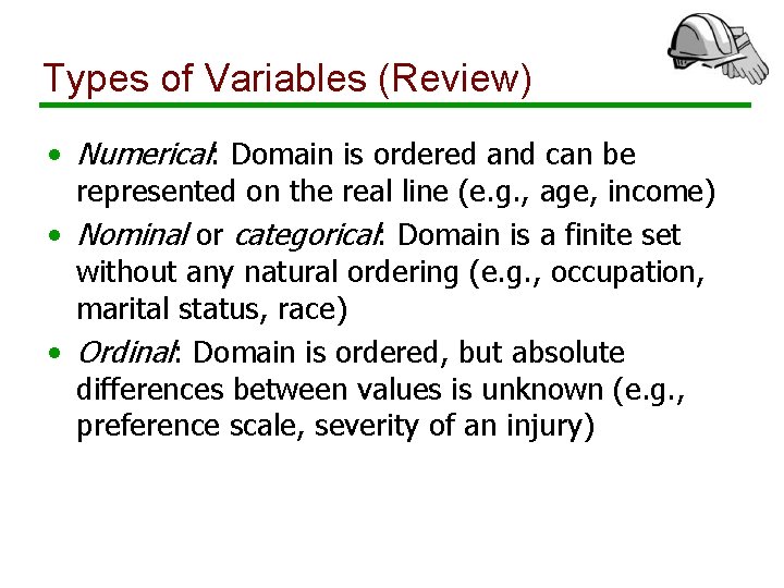
Types of Variables • Numerical: Domain is ordered and can be represented on the real line (e. g. , age, income) • Nominal or categorical: Domain is a finite set without any natural ordering (e. g. , occupation, marital status, race) • Ordinal: Domain is ordered, but absolute differences between values is unknown (e. g. , preference scale, severity of an injury)

Data Mining Techniques • Supervised learning • Classification and regression • Unsupervised learning • Clustering and association rules • Dependency modeling • Outlier and deviation detection • Trend analysis and change detection

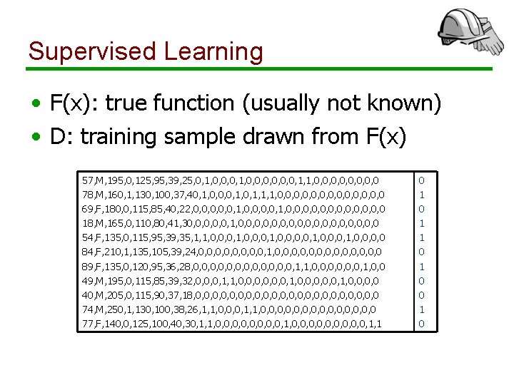
Supervised Learning • F(x): true function (usually not known) • D: training sample drawn from F(x) 57, M, 195, 0, 125, 95, 39, 25, 0, 1, 0, 0, 1, 1, 0, 0, 0, 0 78, M, 160, 1, 130, 100, 37, 40, 1, 0, 0, 0, 1, 1, 1, 0, 0, 0, 0 69, F, 180, 0, 115, 85, 40, 22, 0, 0, 0, 1, 0, 0, 0, 0, 0 18, M, 165, 0, 110, 80, 41, 30, 0, 0, 1, 0, 0, 0, 0, 0 54, F, 135, 0, 115, 95, 39, 35, 1, 1, 0, 0, 0, 1, 0, 0, 0, 0 84, F, 210, 1, 135, 105, 39, 24, 0, 0, 1, 0, 0, 0, 0 89, F, 135, 0, 120, 95, 36, 28, 0, 0, 0, 1, 1, 0, 0, 0, 1, 0, 0 49, M, 195, 0, 115, 85, 39, 32, 0, 0, 0, 1, 1, 0, 0, 0, 1, 0, 0 40, M, 205, 0, 115, 90, 37, 18, 0, 0, 0, 0, 0, 0 74, M, 250, 1, 130, 100, 38, 26, 1, 1, 0, 0, 0, 0, 0 77, F, 140, 0, 125, 100, 40, 30, 1, 1, 0, 0, 0, 0, 0, 1, 1 0 1 1 0 0 1 0

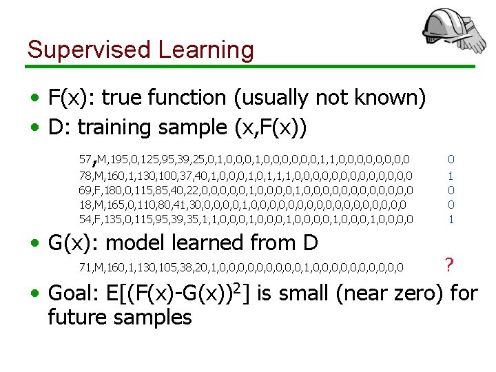
Supervised Learning • F(x): true function (usually not known) • D: training sample (x, F(x)) 57, M, 195, 0, 125, 95, 39, 25, 0, 1, 0, 0, 1, 1, 0, 0, 0, 0 78, M, 160, 1, 130, 100, 37, 40, 1, 0, 0, 0, 1, 1, 1, 0, 0, 0, 0 69, F, 180, 0, 115, 85, 40, 22, 0, 0, 0, 1, 0, 0, 0, 0, 0 18, M, 165, 0, 110, 80, 41, 30, 0, 0, 1, 0, 0, 0, 0, 0 54, F, 135, 0, 115, 95, 39, 35, 1, 1, 0, 0, 0, 1, 0, 0, 0, 0 • G(x): model learned from D 71, M, 160, 1, 130, 105, 38, 20, 1, 0, 0, 0, 0, 0, 0 0 1 ? • Goal: E[(F(x)-G(x))2] is small (near zero) for future samples

Supervised Learning Well-defined goal: Learn G(x) that is a good approximation to F(x) from training sample D Well-defined error metrics: Accuracy, RMSE, ROC, …

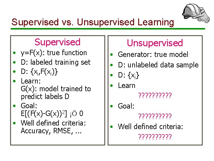
Supervised vs. Unsupervised Learning Supervised • • y=F(x): true function D: labeled training set D: {xi, F(xi)} Learn: G(x): model trained to predict labels D • Goal: E[(F(x)-G(x))2] ¡Ö 0 • Well defined criteria: Accuracy, RMSE, . . . Unsupervised • • Generator: true model D: unlabeled data sample D: {xi} Learn ? ? ? ? ? • Goal: ? ? ? ? ? • Well defined criteria: ? ? ? ? ?

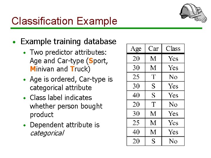
Classification Example • Example training database Two predictor attributes: Age and Car-type (Sport, Minivan and Truck) • Age is ordered, Car-type is categorical attribute • Class label indicates whether person bought product • Dependent attribute is • categorical

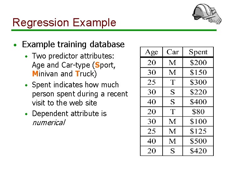
Regression Example • Example training database Two predictor attributes: Age and Car-type (Sport, Minivan and Truck) • Spent indicates how much person spent during a recent visit to the web site • Dependent attribute is • numerical

Types of Variables (Review) • Numerical: Domain is ordered and can be represented on the real line (e. g. , age, income) • Nominal or categorical: Domain is a finite set without any natural ordering (e. g. , occupation, marital status, race) • Ordinal: Domain is ordered, but absolute differences between values is unknown (e. g. , preference scale, severity of an injury)

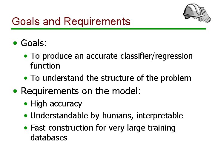
Goals and Requirements • Goals: • To produce an accurate classifier/regression function • To understand the structure of the problem • Requirements on the model: • High accuracy • Understandable by humans, interpretable • Fast construction for very large training databases

Different Types of Classifiers • • Decision Trees Simple Bayesian models Nearest neighbor methods Logistic regression Neural networks Linear discriminant analysis (LDA) Quadratic discriminant analysis (QDA) Density estimation methods

Decision Trees • A decision tree T encodes d (a classifier or regression function) in form of a tree. • A node t in T without children is called a leaf node. Otherwise t is called an internal node.

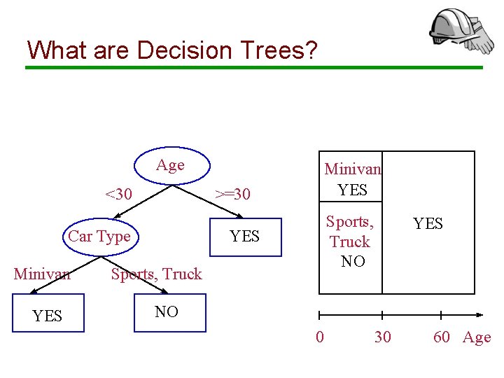
What are Decision Trees? Age <30 >=30 YES Sports, Truck NO YES Car Type Minivan YES Sports, Truck YES NO 0 30 60 Age

Internal Nodes • Each internal node has an associated splitting predicate. Most common are binary predicates. Example predicates: • Age <= 20 • Profession in {student, teacher} • 5000*Age + 3*Salary – 10000 > 0

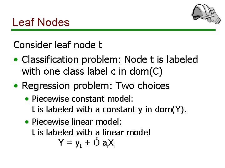
Leaf Nodes Consider leaf node t • Classification problem: Node t is labeled with one class label c in dom(C) • Regression problem: Two choices • Piecewise constant model: t is labeled with a constant y in dom(Y). • Piecewise linear model: t is labeled with a linear model Y = y t + Ó a i. X i

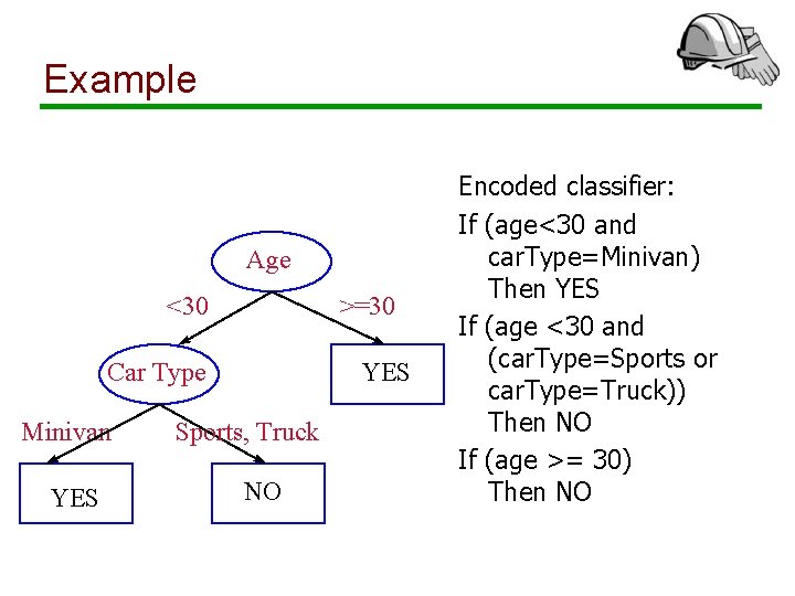
Example Age <30 >=30 YES Car Type Minivan YES Sports, Truck NO Encoded classifier: If (age<30 and car. Type=Minivan) Then YES If (age <30 and (car. Type=Sports or car. Type=Truck)) Then NO If (age >= 30) Then NO

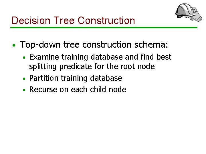
Decision Tree Construction • Top-down tree construction schema: Examine training database and find best splitting predicate for the root node • Partition training database • Recurse on each child node •

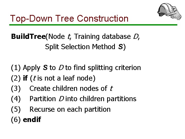
Top-Down Tree Construction Build. Tree(Node t, Training database D, Split Selection Method S) (1) Apply S to D to find splitting criterion (2) if (t is not a leaf node) (3) Create children nodes of t (4) Partition D into children partitions (5) Recurse on each partition (6) endif

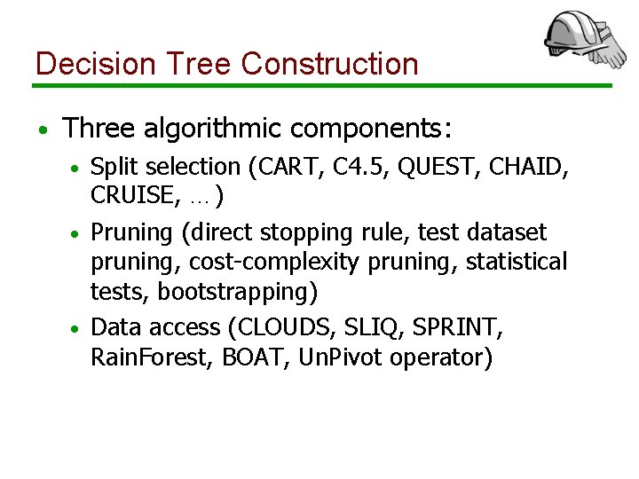
Decision Tree Construction • Three algorithmic components: Split selection (CART, C 4. 5, QUEST, CHAID, CRUISE, …) • Pruning (direct stopping rule, test dataset pruning, cost-complexity pruning, statistical tests, bootstrapping) • Data access (CLOUDS, SLIQ, SPRINT, Rain. Forest, BOAT, Un. Pivot operator) •

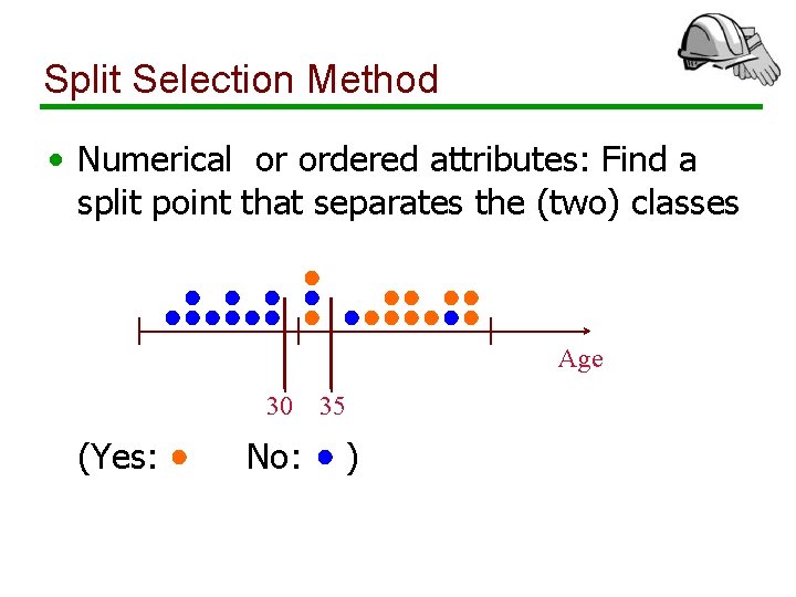
Split Selection Method • Numerical or ordered attributes: Find a split point that separates the (two) classes Age 30 (Yes: No: 35 )

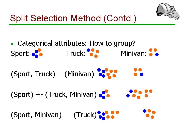
Split Selection Method (Contd. ) Categorical attributes: How to group? Sport: Truck: Minivan: • (Sport, Truck) -- (Minivan) (Sport) --- (Truck, Minivan) (Sport, Minivan) --- (Truck)

Pruning Method • For a tree T, the misclassification rate R(T, P) and the mean-squared error rate R(T, P) depend on P, but not on D. • The goal is to do well on records randomly drawn from P, not to do well on the records in D • If the tree is too large, it overfits D and does not model P. The pruning method selects the tree of the right size.

Data Access Method Recent development: Very large training databases, both in-memory and on secondary storage • Goal: Fast, efficient, and scalable decision tree construction, using the complete training database. •

Decision Trees: Summary • Many application of decision trees • There are many algorithms available for: • • Split selection Pruning Handling Missing Values Data Access • Decision tree construction still active research area (after 20+ years!) • Challenges: Performance, scalability, evolving datasets, new applications

Evaluation of Misclassification Error Problem: • In order to quantify the quality of a classifier d, we need to know its misclassification rate RT(d, P). • But unless we know P, RT(d, P) is unknown. • Thus we need to estimate RT(d, P) as good as possible.

Resubstitution Estimate The Resubstitution estimate R(d, D) estimates RT(d, P) of a classifier d using D: • Let D be the training database with N records. • R(d, D) = 1/N Ó I(d(r. X) != r. C)) • Intuition: R(d, D) is the proportion of training records that is misclassified by d • Problem with resubstitution estimate: Overly optimistic; classifiers that overfit the training dataset will have very low resubstitution error.

Test Sample Estimate • Divide D into D 1 and D 2 • Use D 1 to construct the classifier d • Then use resubstitution estimate R(d, D 2) to calculate the estimated misclassification error of d • Unbiased and efficient, but removes D 2 from training dataset D

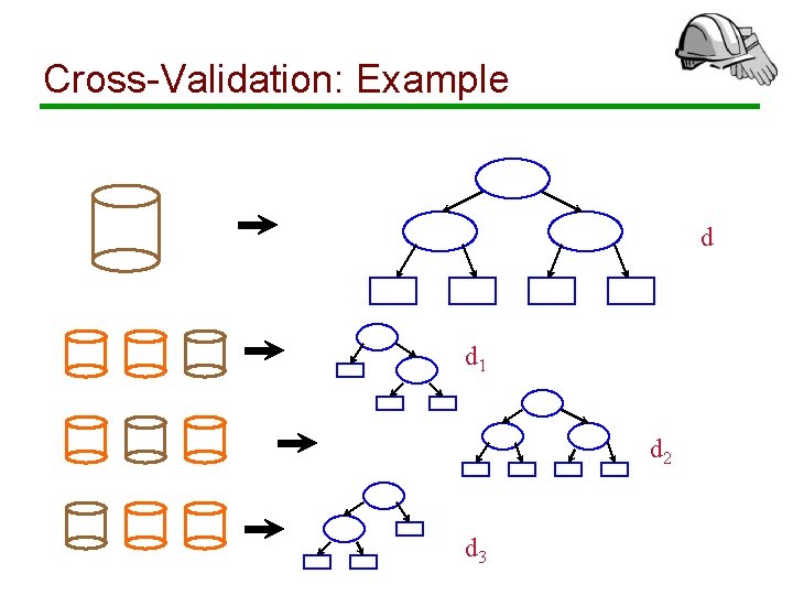
V-fold Cross Validation Procedure: • Construct classifier d from D • Partition D into V datasets D 1, …, DV • Construct classifier di using D Di • Calculate the estimated misclassification error R(di, Di) of di using test sample Di Final misclassification estimate: • Weighted combination of individual misclassification errors: R(d, D) = 1/V Ó R(di, Di)

Cross-Validation: Example d d 1 d 2 d 3

Cross-Validation • Misclassification estimate obtained through cross-validation is usually nearly unbiased • Costly computation (we need to compute d, and d 1, …, d. V); computation of di is nearly as expensive as computation of d • Preferred method to estimate quality of learning algorithms in the machine learning literature

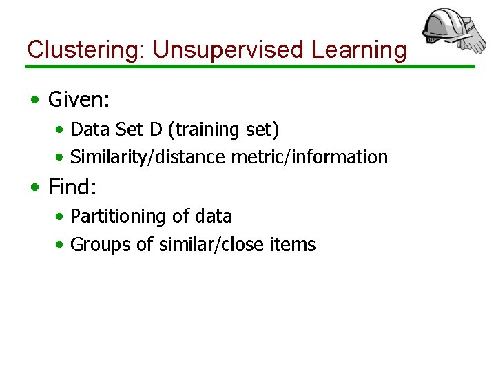
Clustering: Unsupervised Learning • Given: • Data Set D (training set) • Similarity/distance metric/information • Find: • Partitioning of data • Groups of similar/close items

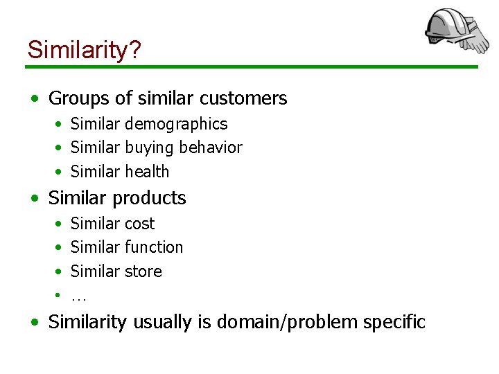
Similarity? • Groups of similar customers • Similar demographics • Similar buying behavior • Similar health • Similar products • • Similar cost Similar function Similar store … • Similarity usually is domain/problem specific

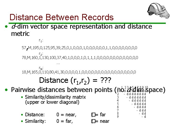
Distance Between Records • d-dim vector space representation and distance metric , r 1: 57 M, 195, 0, 125, 95, 39, 25, 0, 1, 0, 0, 1, 1, 0, 0, 0, 0 r 2: 78, M, 160, 1, 130, 100, 37, 40, 1, 0, 0, 0, 1, 1, 1, 0, 0, 0, 0. . . r. N: 18, M, 165, 0, 110, 80, 41, 30, 0, 0, 1, 0, 0, 0, 0, 0 Distance (r 1, r 2) = ? ? ? -- 1 2 3 4 5 6 7 8 9 10 • Pairwise distances between points (no 1 - dd d d-dim d d dspace) 2 - dddd • Similarity/dissimilarity matrix (upper or lower diagonal) • Distance: • Similarity: 0 = near, 0 = far, ‡�= far ‡ = near � 3 4 5 6 7 8 9 - ddddddd - ddd - d

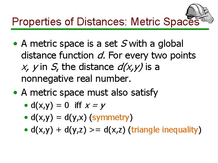
Properties of Distances: Metric Spaces • A metric space is a set S with a global distance function d. For every two points x, y in S, the distance d(x, y) is a nonnegative real number. • A metric space must also satisfy • d(x, y) = 0 iff x = y • d(x, y) = d(y, x) (symmetry) • d(x, y) + d(y, z) >= d(x, z) (triangle inequality)

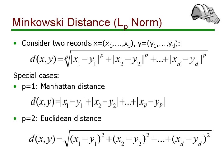
Minkowski Distance (Lp Norm) • Consider two records x=(x 1, …, xd), y=(y 1, …, yd): Special cases: • p=1: Manhattan distance • p=2: Euclidean distance

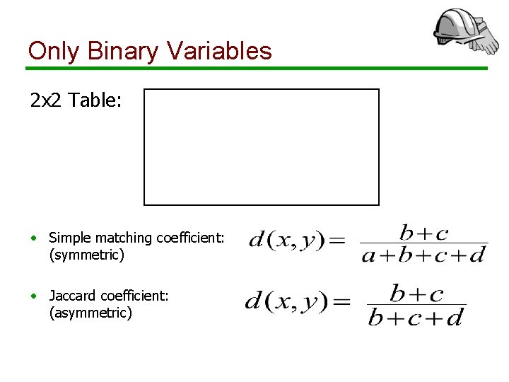
Only Binary Variables 2 x 2 Table: • Simple matching coefficient: (symmetric) • Jaccard coefficient: (asymmetric)

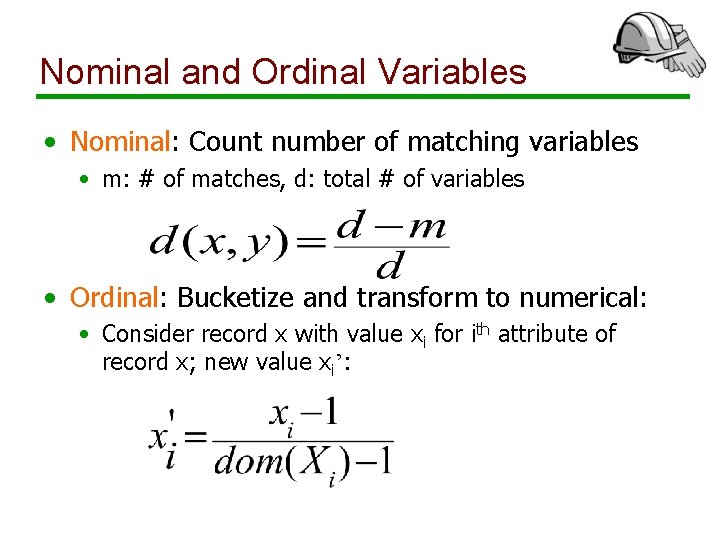
Nominal and Ordinal Variables • Nominal: Count number of matching variables • m: # of matches, d: total # of variables • Ordinal: Bucketize and transform to numerical: • Consider record x with value xi for ith attribute of record x; new value xi’:

Mixtures of Variables • Weigh each variable differently • Can take “importance” of variable into account (although usually hard to quantify in practice)

Clustering: Informal Problem Definition Input: • A data set of N records each given as a ddimensional data feature vector. Output: • Determine a natural, useful “partitioning” of the data set into a number of (k) clusters and noise such that we have: • High similarity of records within each cluster (intracluster similarity) • Low similarity of records between clusters (intercluster similarity)

Types of Clustering • Hard Clustering: • Each object is in one and only one cluster • Soft Clustering: • Each object has a probability of being in each cluster

Clustering Algorithms • Partitioning-based clustering • K-means clustering • K-medoids clustering • EM (expectation maximization) clustering • Hierarchical clustering • Divisive clustering (top down) • Agglomerative clustering (bottom up) • Density-Based Methods • Regions of dense points separated by sparser regions of relatively low density

K-Means Clustering Algorithm Initialize k cluster centers Do Assignment step: Assign each data point to its closest cluster center Re-estimation step: Re-compute cluster centers While (there are still changes in the cluster centers) Visualization at: • http: //www. delft-cluster. nl/textminer/theory/kmeans. html

Issues Why is K-Means working: • How does it find the cluster centers? • Does it find an optimal clustering • What are good starting points for the algorithm? • What is the right number of cluster centers? • How do we know it will terminate?

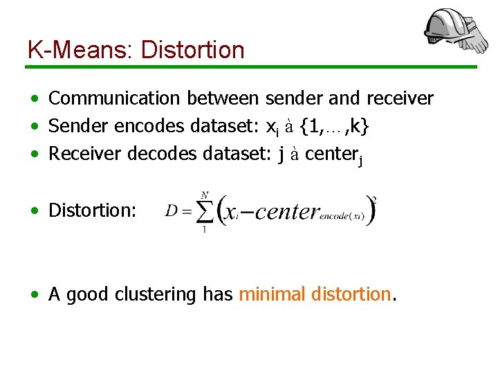
K-Means: Distortion • Communication between sender and receiver • Sender encodes dataset: xi à {1, …, k} • Receiver decodes dataset: j à centerj • Distortion: • A good clustering has minimal distortion.

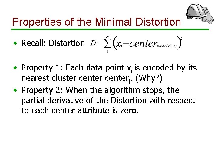
Properties of the Minimal Distortion • Recall: Distortion • Property 1: Each data point xi is encoded by its nearest cluster centerj. (Why? ) • Property 2: When the algorithm stops, the partial derivative of the Distortion with respect to each center attribute is zero.

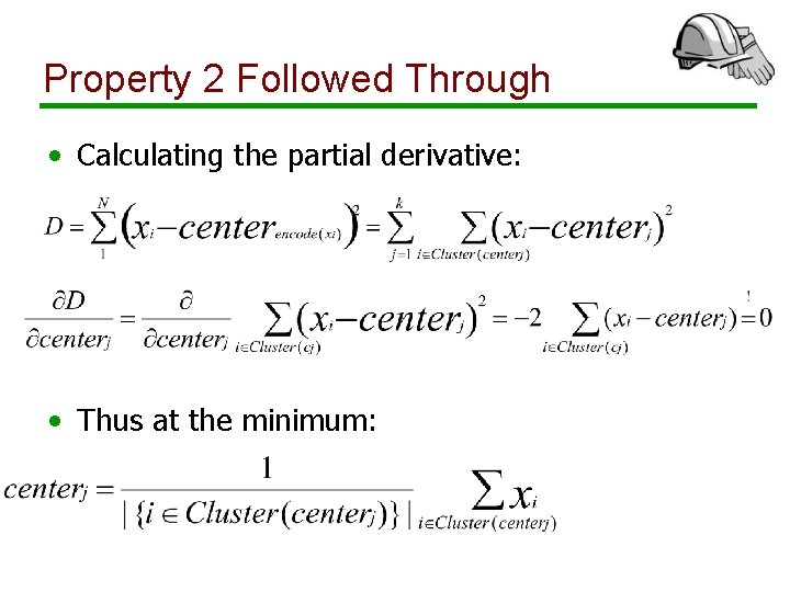
Property 2 Followed Through • Calculating the partial derivative: • Thus at the minimum:

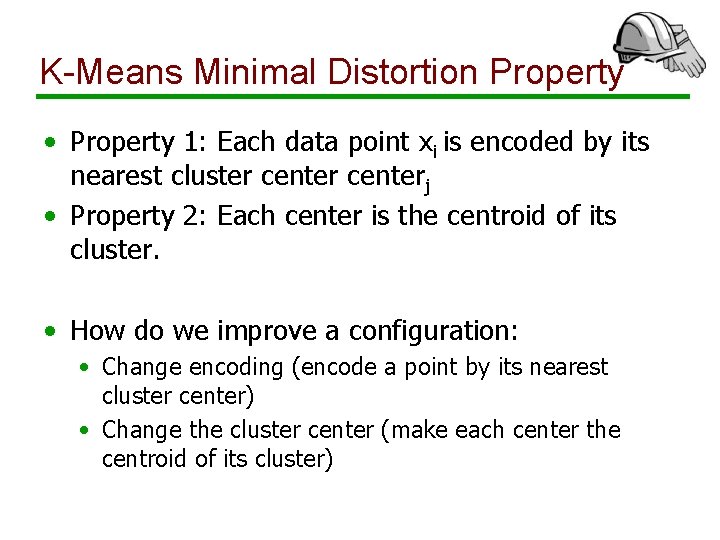
K-Means Minimal Distortion Property • Property 1: Each data point xi is encoded by its nearest cluster centerj • Property 2: Each center is the centroid of its cluster. • How do we improve a configuration: • Change encoding (encode a point by its nearest cluster center) • Change the cluster center (make each center the centroid of its cluster)

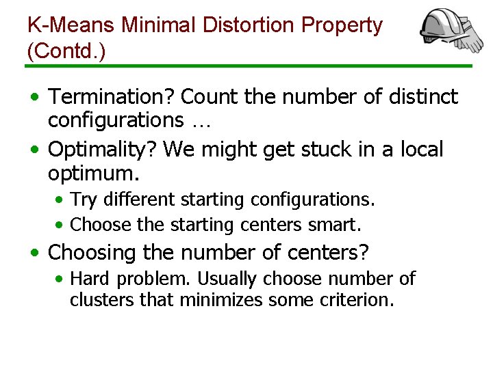
K-Means Minimal Distortion Property (Contd. ) • Termination? Count the number of distinct configurations … • Optimality? We might get stuck in a local optimum. • Try different starting configurations. • Choose the starting centers smart. • Choosing the number of centers? • Hard problem. Usually choose number of clusters that minimizes some criterion.

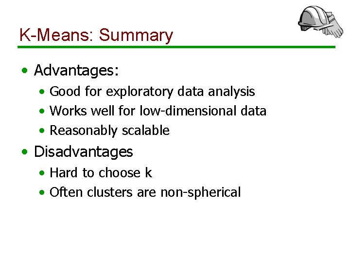
K-Means: Summary • Advantages: • Good for exploratory data analysis • Works well for low-dimensional data • Reasonably scalable • Disadvantages • Hard to choose k • Often clusters are non-spherical

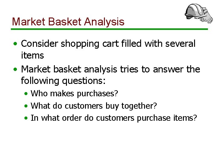
Market Basket Analysis • Consider shopping cart filled with several items • Market basket analysis tries to answer the following questions: • Who makes purchases? • What do customers buy together? • In what order do customers purchase items?

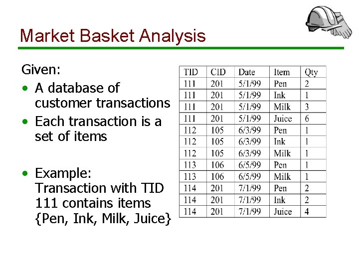
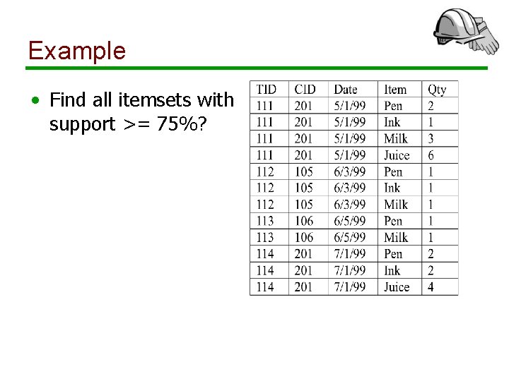
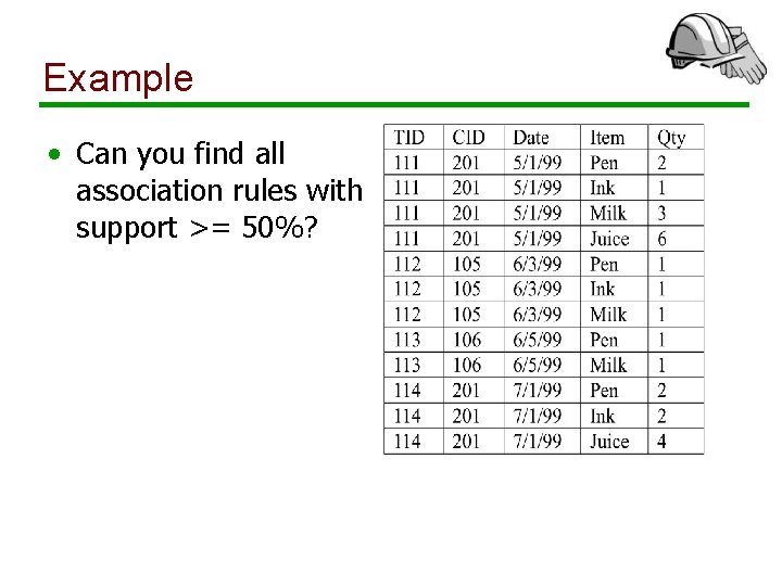
Market Basket Analysis Given: • A database of customer transactions • Each transaction is a set of items • Example: Transaction with TID 111 contains items {Pen, Ink, Milk, Juice}

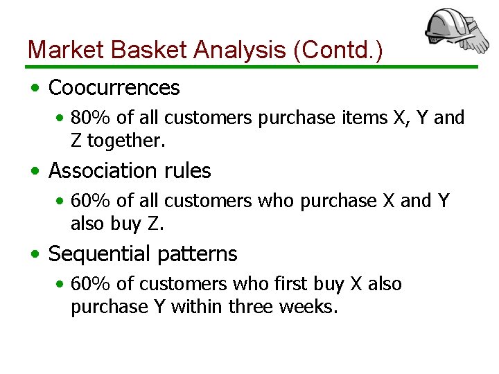
Market Basket Analysis (Contd. ) • Coocurrences • 80% of all customers purchase items X, Y and Z together. • Association rules • 60% of all customers who purchase X and Y also buy Z. • Sequential patterns • 60% of customers who first buy X also purchase Y within three weeks.

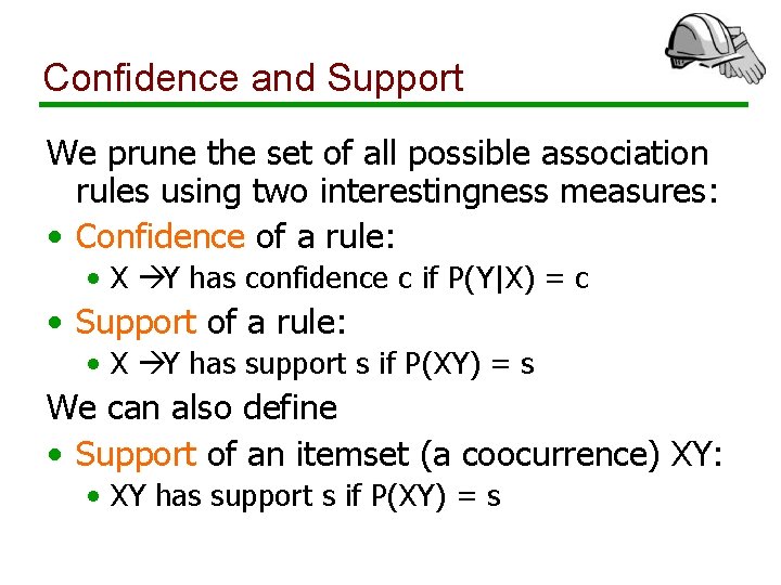
Confidence and Support We prune the set of all possible association rules using two interestingness measures: • Confidence of a rule: • X Y has confidence c if P(Y|X) = c • Support of a rule: • X Y has support s if P(XY) = s We can also define • Support of an itemset (a coocurrence) XY: • XY has support s if P(XY) = s

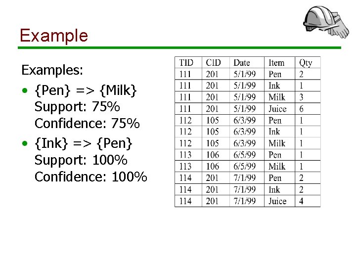
Examples: • {Pen} => {Milk} Support: 75% Confidence: 75% • {Ink} => {Pen} Support: 100% Confidence: 100%

Example • Find all itemsets with support >= 75%?

Example • Can you find all association rules with support >= 50%?

Market Basket Analysis: Applications • Sample Applications • • • Direct marketing Fraud detection for medical insurance Floor/shelf planning Web site layout Cross-selling

Applications of Frequent Itemsets • Market Basket Analysis • Association Rules • Classification (especially: text, rare classes) • Seeds for construction of Bayesian Networks • Web log analysis • Collaborative filtering

Association Rule Algorithms • More abstract problem redux • Breadth-first search • Depth-first search

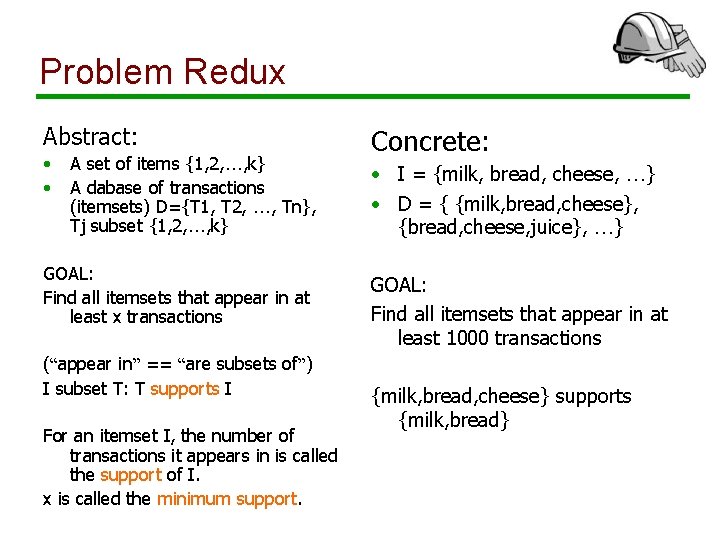
Problem Redux Abstract: • • A set of items {1, 2, …, k} A dabase of transactions (itemsets) D={T 1, T 2, …, Tn}, Tj subset {1, 2, …, k} GOAL: Find all itemsets that appear in at least x transactions (“appear in” == “are subsets of”) I subset T: T supports I For an itemset I, the number of transactions it appears in is called the support of I. x is called the minimum support. Concrete: • I = {milk, bread, cheese, …} • D = { {milk, bread, cheese}, {bread, cheese, juice}, …} GOAL: Find all itemsets that appear in at least 1000 transactions {milk, bread, cheese} supports {milk, bread}

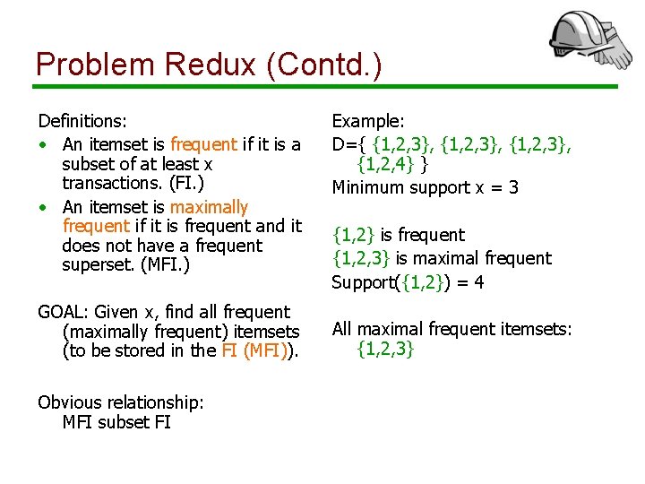
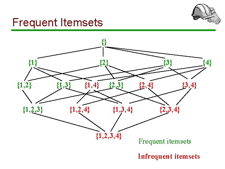
Problem Redux (Contd. ) Definitions: • An itemset is frequent if it is a subset of at least x transactions. (FI. ) • An itemset is maximally frequent if it is frequent and it does not have a frequent superset. (MFI. ) GOAL: Given x, find all frequent (maximally frequent) itemsets (to be stored in the FI (MFI)). Obvious relationship: MFI subset FI Example: D={ {1, 2, 3}, {1, 2, 4} } Minimum support x = 3 {1, 2} is frequent {1, 2, 3} is maximal frequent Support({1, 2}) = 4 All maximal frequent itemsets: {1, 2, 3}

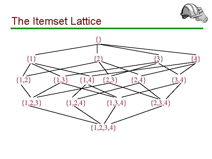
The Itemset Lattice {} {1, 2} {1, 2, 3} {2} {1, 3} {1, 4} {1, 2, 4} {3} {2, 3} {1, 3, 4} {1, 2, 3, 4} {2, 4} {3, 4} {2, 3, 4}

Frequent Itemsets {} {1, 2} {1, 2, 3} {2} {1, 3} {1, 4} {1, 2, 4} {3} {2, 3} {1, 3, 4} {1, 2, 3, 4} {2, 4} {3, 4} {2, 3, 4} Frequent itemsets Infrequent itemsets

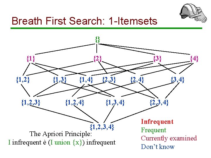
Breath First Search: 1 -Itemsets {} {1, 2} {1, 2, 3} {2} {1, 3} {1, 4} {1, 2, 4} {3} {2, 3} {1, 3, 4} {1, 2, 3, 4} The Apriori Principle: I infrequent è (I union {x}) infrequent {2, 4} {3, 4} {2, 3, 4} Infrequent Frequent Currently examined Don’t know

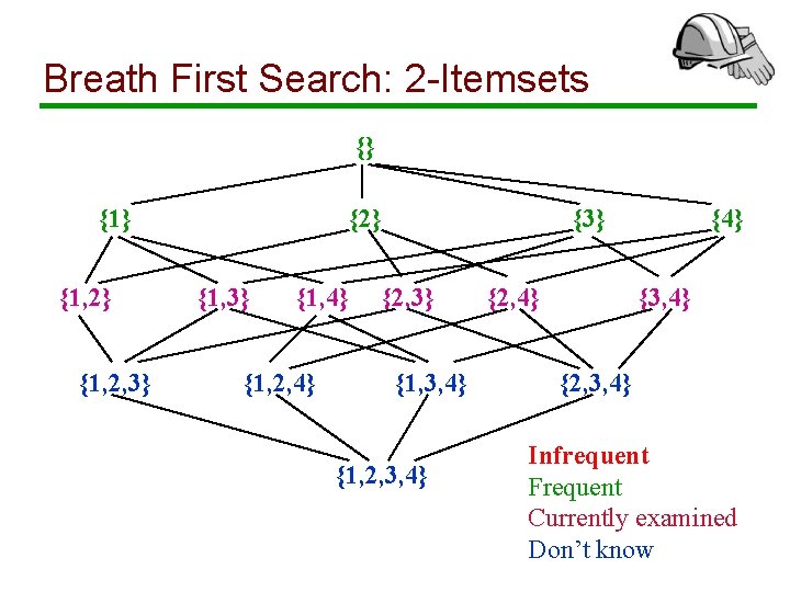
Breath First Search: 2 -Itemsets {} {1, 2} {1, 2, 3} {2} {1, 3} {1, 4} {1, 2, 4} {3} {2, 3} {1, 3, 4} {1, 2, 3, 4} {2, 4} {3, 4} {2, 3, 4} Infrequent Frequent Currently examined Don’t know

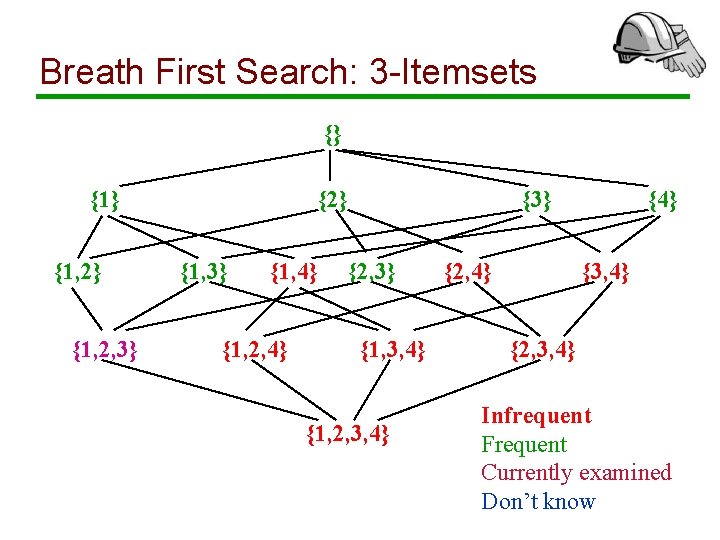
Breath First Search: 3 -Itemsets {} {1, 2} {1, 2, 3} {2} {1, 3} {1, 4} {1, 2, 4} {3} {2, 3} {1, 3, 4} {1, 2, 3, 4} {2, 4} {3, 4} {2, 3, 4} Infrequent Frequent Currently examined Don’t know

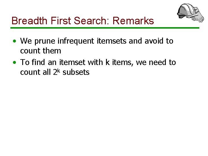
Breadth First Search: Remarks • We prune infrequent itemsets and avoid to count them • To find an itemset with k items, we need to count all 2 k subsets

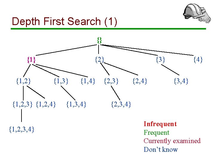
Depth First Search (1) {} {1, 2} {1, 3} {1, 2, 4} {1, 2, 3, 4} {1, 3, 4} {3} {2, 4} {3, 4} {2, 3, 4} Infrequent Frequent Currently examined Don’t know

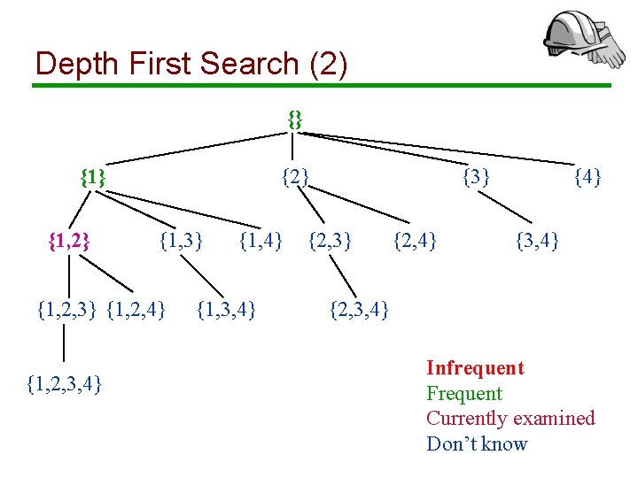
Depth First Search (2) {} {1, 2} {1, 3} {1, 2, 4} {1, 2, 3, 4} {1, 3, 4} {3} {2, 4} {3, 4} {2, 3, 4} Infrequent Frequent Currently examined Don’t know

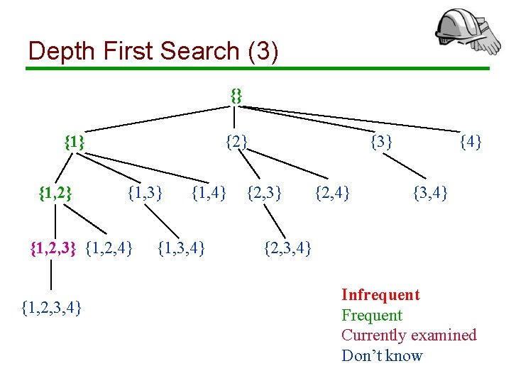
Depth First Search (3) {} {1, 2} {1, 3} {1, 2, 4} {1, 2, 3, 4} {1, 3, 4} {3} {2, 4} {3, 4} {2, 3, 4} Infrequent Frequent Currently examined Don’t know

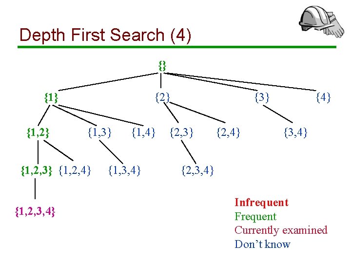
Depth First Search (4) {} {1, 2} {1, 3} {1, 2, 4} {1, 2, 3, 4} {1, 3, 4} {3} {2, 4} {3, 4} {2, 3, 4} Infrequent Frequent Currently examined Don’t know

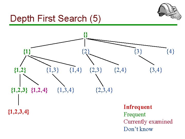
Depth First Search (5) {} {1, 2} {1, 3} {1, 2, 4} {1, 2, 3, 4} {1, 3, 4} {3} {2, 4} {3, 4} {2, 3, 4} Infrequent Frequent Currently examined Don’t know

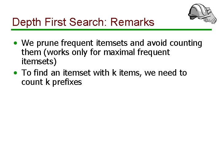
Depth First Search: Remarks • We prune frequent itemsets and avoid counting them (works only for maximal frequent itemsets) • To find an itemset with k items, we need to count k prefixes

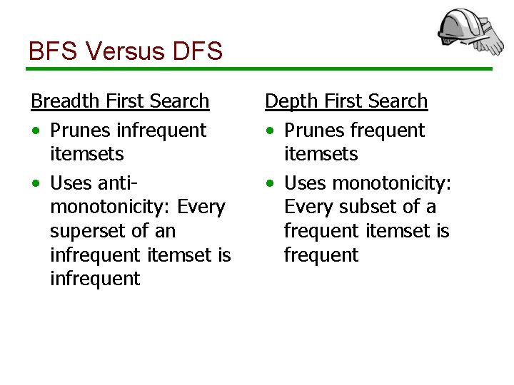
BFS Versus DFS Breadth First Search • Prunes infrequent itemsets • Uses antimonotonicity: Every superset of an infrequent itemset is infrequent Depth First Search • Prunes frequent itemsets • Uses monotonicity: Every subset of a frequent itemset is frequent

Extensions • Imposing constraints • • Only find rules involving the dairy department Only find rules involving expensive products Only find “expensive” rules Only find rules with “whiskey” on the right hand side Only find rules with “milk” on the left hand side Hierarchies on the items Calendars (every Sunday, every 1 st of the month)

Itemset Constraints Definition: • A constraint is an arbitrary property of itemsets. Examples: • The itemset has support greater than 1000. • No element of the itemset costs more than $40. • The items in the set average more than $20. Goal: • Find all itemsets satisfying a given constraint P. “Solution”: • If P is a support constraint, use the Apriori Algorithm.