Chapter 23 Model Based Algorithms Figure 1 Model
Chapter 23 Model Based Algorithms

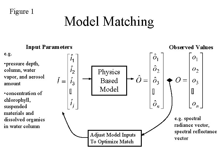
Figure 1 Model Matching Input Parameters Observed Values e. g. • pressure depth, column, water vapor, and aerosol amount • concentration of chlorophyll, suspended materials and dissolved organics in water column Physics Based Model Adjust Model Inputs To Optimize Match e. g. spectral radiance vector, spectral reflectance vector
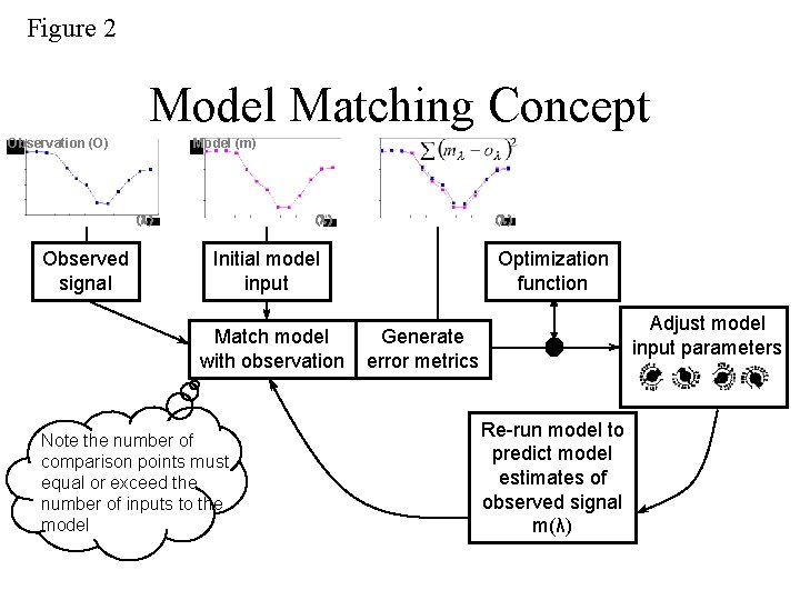
Figure 2 Model Matching Concept Observation (O) Model (m) (l) Observed signal (l) Initial model input Match model with observation Note the number of comparison points must equal or exceed the number of inputs to the model Optimization function Adjust model input parameters Generate error metrics Re-run model to predict model estimates of observed signal m(λ)
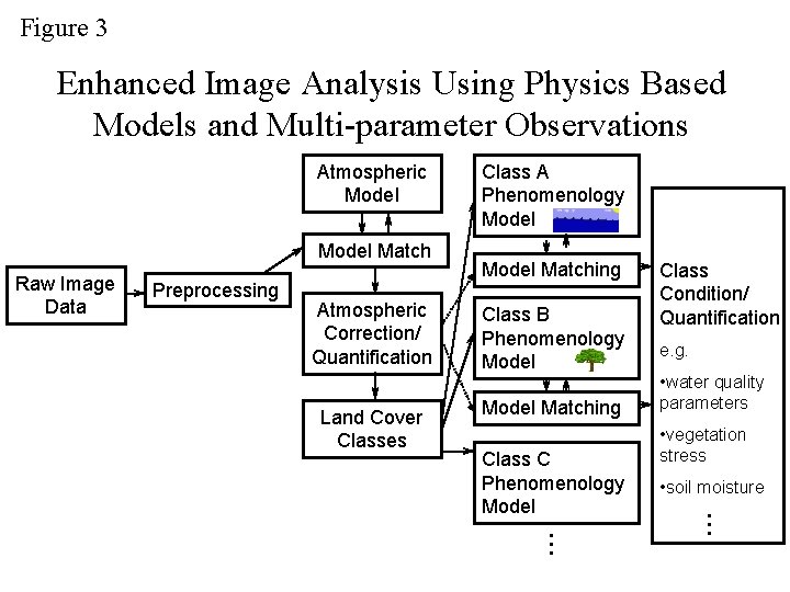
Figure 3 Enhanced Image Analysis Using Physics Based Models and Multi-parameter Observations Atmospheric Model Match Raw Image Data Preprocessing Atmospheric Correction/ Quantification Land Cover Classes Class A Phenomenology Model Matching Class B Phenomenology Model Matching e. g. • water quality parameters • vegetation stress • soil moisture ¼ ¼ Class C Phenomenology Model Class Condition/ Quantification

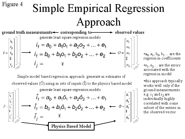
Figure 4 Simple Empirical Regression Approach ground truth measurements corresponding to observed values generate least square regression models <m > • a 0, a 1, b 0, b 1… are the regression coefficients Simple model based regression approach: generate m estimates of observed values (Ô) using m sets of inputs (Î) to the physics based model Physics Based Model <m > generate least square regression models • e 1, e 2… are the errors associated with the regression model • this approach typically works well only if the ground measurements e. g. i 1 and i 2 are individually highly correlated with some subset of the entries in the observed vector
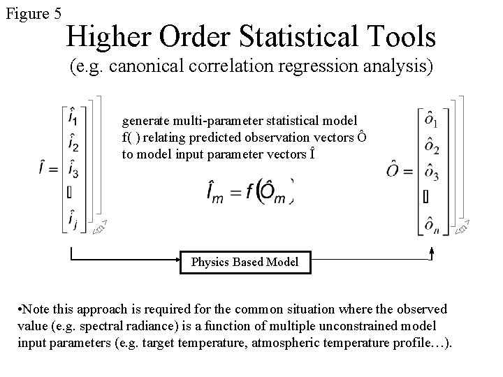
Figure 5 Higher Order Statistical Tools (e. g. canonical correlation regression analysis) <m > generate multi-parameter statistical model f( ) relating predicted observation vectors Ô to model input parameter vectors Î Physics Based Model • Note this approach is required for the common situation where the observed value (e. g. spectral radiance) is a function of multiple unconstrained model input parameters (e. g. target temperature, atmospheric temperature profile…).

Figure 6 Use of Physics Based Models for Training Algorithms Samples of Training Class A e. g. trees Physics Based Model <m > Database of measurements of model inputs that describes Class A Class B e. g. road <m > Physics Based Model <m > Database of measurements of model inputs that describes Class B Parametric or Non-parametric C L A S S I F I E R Classification procedures for any vector of the form
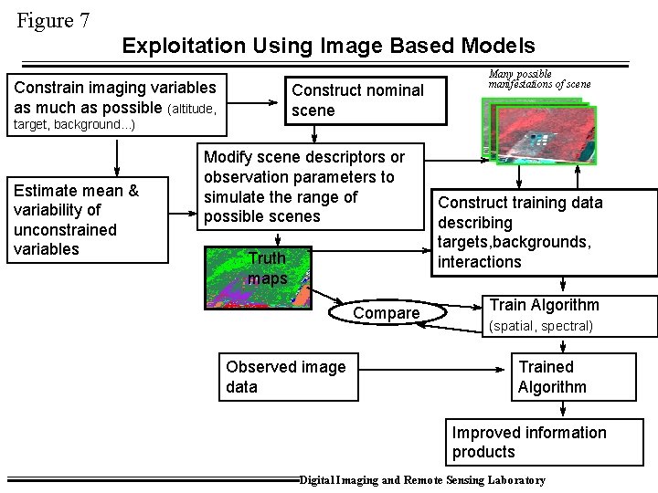
Figure 7 Exploitation Using Image Based Models Constrain imaging variables as much as possible (altitude, Construct nominal scene target, background. . . ) Estimate mean & variability of unconstrained variables Modify scene descriptors or observation parameters to simulate the range of possible scenes Truth maps Compare Observed image data Many possible manifestations of scene Construct training data describing targets, backgrounds, interactions Train Algorithm (spatial, spectral) Trained Algorithm Improved information products Digital Imaging and Remote Sensing Laboratory
- Slides: 10