Chapter 22 The Demand for Money Quantity Theory

Chapter 22 The Demand for Money

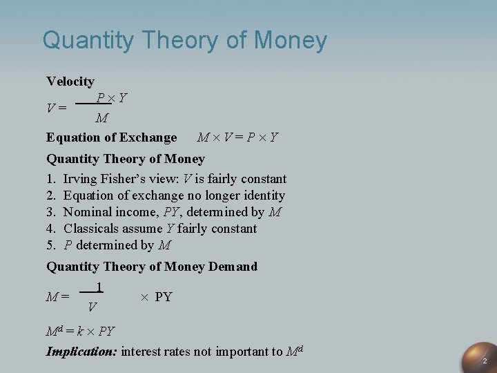
Quantity Theory of Money Velocity P Y M Equation of Exchange V= M V=P Y Quantity Theory of Money 1. Irving Fisher’s view: V is fairly constant 2. Equation of exchange no longer identity 3. Nominal income, PY, determined by M 4. Classicals assume Y fairly constant 5. P determined by M Quantity Theory of Money Demand 1 M= PY V Md = k PY Implication: interest rates not important to Md 2

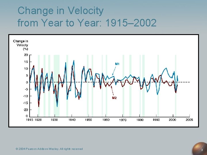
Change in Velocity from Year to Year: 1915– 2002 © 2004 Pearson Addison-Wesley. All rights reserved 3

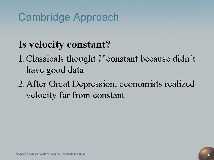
Cambridge Approach Is velocity constant? 1. Classicals thought V constant because didn’t have good data 2. After Great Depression, economists realized velocity far from constant © 2004 Pearson Addison-Wesley. All rights reserved 4

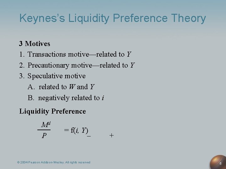
Keynes’s Liquidity Preference Theory 3 Motives 1. Transactions motive—related to Y 2. Precautionary motive—related to Y 3. Speculative motive A. related to W and Y B. negatively related to i Liquidity Preference Md P = f(i, Y) – © 2004 Pearson Addison-Wesley. All rights reserved + 5

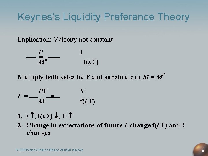
Keynes’s Liquidity Preference Theory Implication: Velocity not constant P =d M 1 f(i, Y) Multiply both sides by Y and substitute in M = Md V= PY = M Y f(i, Y) 1. i , f(i, Y) , V 2. Change in expectations of future i, change f(i, Y) and V changes © 2004 Pearson Addison-Wesley. All rights reserved 6

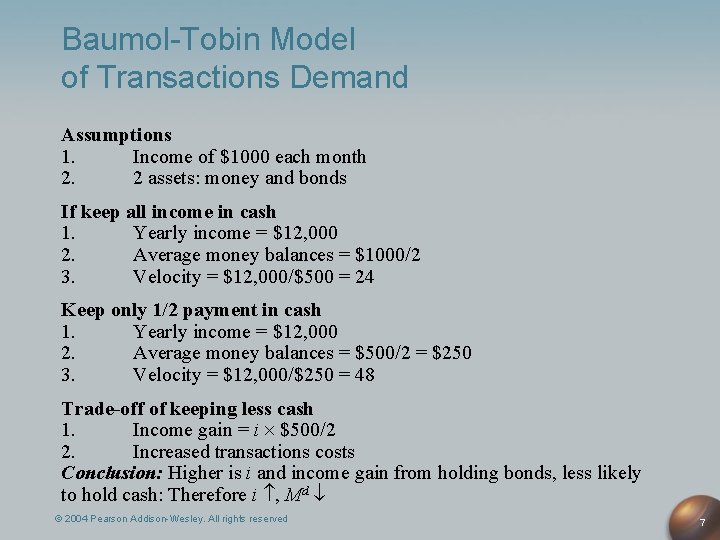
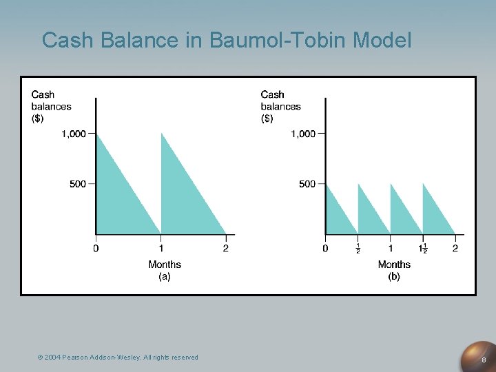
Baumol-Tobin Model of Transactions Demand Assumptions 1. Income of $1000 each month 2. 2 assets: money and bonds If keep all income in cash 1. Yearly income = $12, 000 2. Average money balances = $1000/2 3. Velocity = $12, 000/$500 = 24 Keep only 1/2 payment in cash 1. Yearly income = $12, 000 2. Average money balances = $500/2 = $250 3. Velocity = $12, 000/$250 = 48 Trade-off of keeping less cash 1. Income gain = i $500/2 2. Increased transactions costs Conclusion: Higher is i and income gain from holding bonds, less likely to hold cash: Therefore i , Md © 2004 Pearson Addison-Wesley. All rights reserved 7

Cash Balance in Baumol-Tobin Model © 2004 Pearson Addison-Wesley. All rights reserved 8

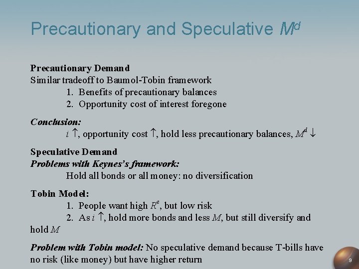
Precautionary and Speculative Md Precautionary Demand Similar tradeoff to Baumol-Tobin framework 1. Benefits of precautionary balances 2. Opportunity cost of interest foregone Conclusion: i , opportunity cost , hold less precautionary balances, Md Speculative Demand Problems with Keynes’s framework: Hold all bonds or all money: no diversification Tobin Model: 1. People want high Re, but low risk 2. As i , hold more bonds and less M, but still diversify and hold M Problem with Tobin model: No speculative demand because T-bills have no risk (like money) but have higher return 9

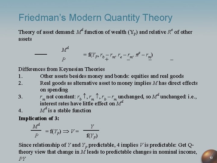
Friedman’s Modern Quantity Theory of asset demand: Md function of wealth (YP) and relative Re of other assets Md P = f(YP, rb – rm, re – rm, e – rm) + – – – Differences from Keynesian Theories 1. Other assets besides money and bonds: equities and real goods 2. Real goods as alternative asset to money implies M has direct effects on spending 3. rm not constant: rb , rm , rb – rm unchanged, so Md unchanged: i. e. , interest rates have little effect on Md 4. Md is a stable function Implication of 3: Md Y = f(YP) V = P f(YP) Since relationship of Y and YP predictable, 4 implies V is predictable: Get Qtheory view that change in M leads to predictable changes in nominal income, PY 10

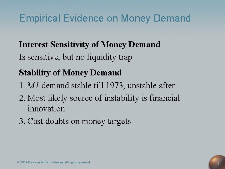
Empirical Evidence on Money Demand Interest Sensitivity of Money Demand Is sensitive, but no liquidity trap Stability of Money Demand 1. M 1 demand stable till 1973, unstable after 2. Most likely source of instability is financial innovation 3. Cast doubts on money targets © 2004 Pearson Addison-Wesley. All rights reserved 11