Chapter 22 Chisquare test for twoway tables R
Chapter 22: Chi-square test for two-way tables R code example Copyright © 2018 W. H. Freeman and Company
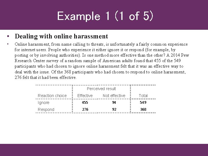
Example 1 (1 of 5) • Dealing with online harassment • Online harassment, from name calling to threats, is unfortunately a fairly common experience for internet users. People who experience it either ignore it or respond (for example, by posting or by involving authorities). Is one method more effective than the other? A 2014 Pew Research Center survey of a random sample of American adults found that 455 of the 549 participants who had chosen to ignore online harassment felt that it was an effective way to deal with the issue. Of the 368 participants who had chosen to respond to online harassment, 276 felt that it had been effective. Perceived result Reaction choice Effective Not effective Total Ignore 455 94 549 Respond 276 92 368
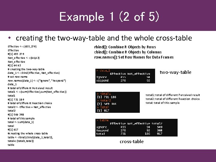
Example 1 (2 of 5) • creating the two-way-table and the whole cross-table Effective <- c(455, 276) Effective #[1] 455 276 Not_effective <- c(94, 92) Not_effective #[1] 94 92 # creating the two-way-table data_1 <- cbind(Effective, Not_effective) # set row name row. names(data_1) <- c("Ignore", "Respond") data_1 # total of different Perceived result total 1 <- c(sum(Effective), sum(Not_effective)) total 1 #[1] 731 186 # total of different Reaction choice total 2 <- Effective + Not_effective total 2 #[1] 549 368 # total of this sample total <- sum(data_1) total #[1] 917 #creating the whole cross-table <- rbind(cbind(data_1, total 2), total=c(total 1, total)) table rbind(): Combine R Objects by Rows cbind(): Combine R Objects by Columns row. names(): Set Row Names for Data Frames two-way-table total 1: total of different Perceived result total 2: total of different Reaction choice total: total of this sample cross-table
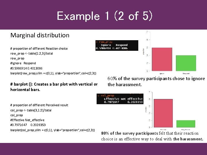
Example 1 (2 of 5) Marginal distribution # proportion of different Reaction choice row_prop <- table[1: 2, 3]/total row_prop #Ignore Respond #0. 5986914 0. 4013086 barplot(row_prop, ylim = c(0, 1), ylab="proportion", col=c(2, 3)) # barplot (): Creates a bar plot with vertical or horizontal bars. # proportion of different Perceived result col_prop <- table[3, 1: 2]/total col_prop #Effective Not_effective #0. 7971647 0. 2028353 barplot(col_prop, ylim = c(0, 1), ylab="proportion", col=c(2, 3)) 60% of the survey participants chose to ignore the harassment. 80% of the survey participants felt that their reaction choice is an effective way to deal with the harassment.
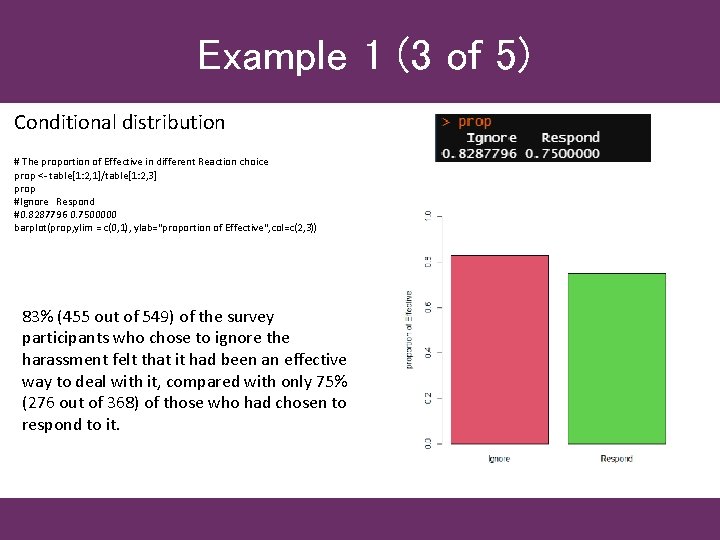
Example 1 (3 of 5) Conditional distribution # The proportion of Effective in different Reaction choice prop <- table[1: 2, 1]/table[1: 2, 3] prop #Ignore Respond #0. 8287796 0. 7500000 barplot(prop, ylim = c(0, 1), ylab="proportion of Effective", col=c(2, 3)) 83% (455 out of 549) of the survey participants who chose to ignore the harassment felt that it had been an effective way to deal with it, compared with only 75% (276 out of 368) of those who had chosen to respond to it.
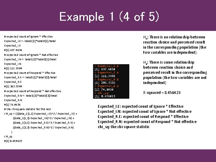
Example 1 (4 of 5) # expected count of Ignore * Effective Expected_I. E <- total 1[1]*total 2[1]/total Expected_I. E #[1] 437. 6434 # expected count of Ignore * Not effective Expected_I. N <- total 1[2]*total 2[1]/total Expected_I. N #[1] 111. 3566 # expected count of Respond * Effective Expected_R. E <- total 1[1]*total 2[2]/total Expected_R. E #[1] 293. 3566 # expected count of Respond * Not effective Expected_R. N <- total 1[2]*total 2[2]/total Expected_R. N #[1] 74. 6434 # the chi-square statistic for this test chi_sq <-(((data_1[1, 1]-Expected_I. E)^2 / Expected_I. E) + ((data_1[1, 2]-Expected_I. N)^2 / Expected_I. N) + ((data_1[2, 1]-Expected_R. E)^2 / Expected_R. E) + ((data_1[2, 2]-Expected_R. N)^2 / Expected_R. N) ) chi_sq #[1] 8. 456423 H 0: There is no relationship between reaction choice and perceived result in the corresponding population (the two variables are independent). Ha: There is some relationship between reaction choice and perceived result in the corresponding population (the two variables are not independent) X-squared = 8. 456423 Expected_I. E: expected count of Ignore * Effective Expected_I. N: expected count of Ignore * Not effective Expected_R. E: expected count of Respond * Effective Expected_R. N: expected count of Respond * Not effective chi_sq: the chi-square statistic
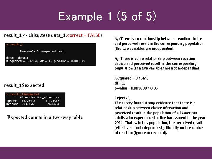
Example 1 (5 of 5) result_1 <- chisq. test(data_1, correct = FALSE) H 0: There is no relationship between reaction choice and perceived result in the corresponding population (the two variables are independent). Ha: There is some relationship between reaction choice and perceived result in the corresponding population (the two variables are not independent) result_1$expected Expected counts in a two-way table X-squared = 8. 4564, df = 1, p-value = 0. 003638 < 0. 05 Reject H 0 The survey found strong evidence that there is a relationship between choice of reaction and perceived result in the population of all American adults who experienced online harassment in the year 2014. That is, in this population, the perceived result (effective or not) depends significantly on the choice of reaction (ignore or respond).
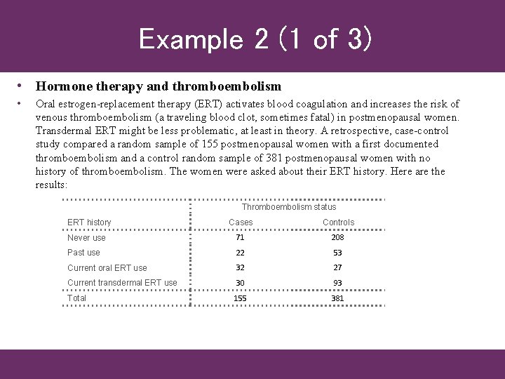
Example 2 (1 of 3) • Hormone therapy and thromboembolism • Oral estrogen-replacement therapy (ERT) activates blood coagulation and increases the risk of venous thromboembolism (a traveling blood clot, sometimes fatal) in postmenopausal women. Transdermal ERT might be less problematic, at least in theory. A retrospective, case-control study compared a random sample of 155 postmenopausal women with a first documented thromboembolism and a control random sample of 381 postmenopausal women with no history of thromboembolism. The women were asked about their ERT history. Here are the results: Thromboembolism status ERT history Cases Controls Never use 71 208 Past use 22 53 Current oral ERT use 32 27 Current transdermal ERT use 30 93 Total 155 381
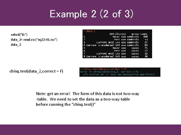
Example 2 (2 of 3) setwd("D: ") data_2<-read. csv("eg 22 -01. csv") data_2 chisq. test(data_2, correct = F) Note: get an error! The form of this data is not two-way -table. We need to set the data as a two-way-table before running the “chisq. test()”
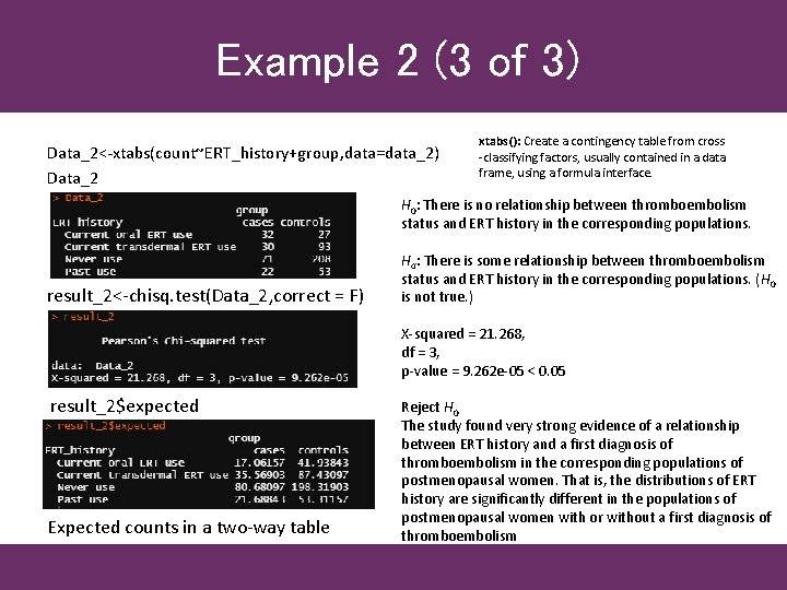
Example 2 (3 of 3) Data_2<-xtabs(count~ERT_history+group, data=data_2) Data_2 xtabs(): Create a contingency table from cross -classifying factors, usually contained in a data frame, using a formula interface. H 0: There is no relationship between thromboembolism status and ERT history in the corresponding populations. result_2<-chisq. test(Data_2, correct = F) Ha: There is some relationship between thromboembolism status and ERT history in the corresponding populations. (H 0 is not true. ) X-squared = 21. 268, df = 3, p-value = 9. 262 e-05 < 0. 05 result_2$expected Expected counts in a two-way table Reject H 0 The study found very strong evidence of a relationship between ERT history and a first diagnosis of thromboembolism in the corresponding populations of postmenopausal women. That is, the distributions of ERT history are significantly different in the populations of postmenopausal women with or without a first diagnosis of thromboembolism
Covid-19 Example (1 of 5) • Coronavirus disease 2019 an infectious disease caused by severe acute respiratory syndrome coronavirus 2 (SARS-Co. V-2). Data sources 1: COVID-19 Data Repository by the Center for Systems Science and Engineering (CSSE) at Johns Hopkins University. https: //github. com/CSSEGISand. Data/COVID-19/tree/master/csse_covid_19_data Data sources 2: United States by Population Density 2020 https: //worldpopulationreview. com/state-rankings/state-densities Whether the Population Density of the United States has a relationship with the severity of Covid-19? In chapter 20, we know that the positive test rates is influenced greatly by the size of tested. So, here we use Mortality Rate to evaluate the severity of Covid-19.
Covid-19 Example (2 of 5) Data file: 09 -26 -2020. csv • https: //github. com/CSSEGISand. Data/COVID-19/tree/master/csse_covid_19_data/csse_covid_19_daily_reports_us USA daily state reports (csse_covid_19_daily_reports_us ) • This table contains an aggregation of each USA State level data. File naming convention • MM-DD-YYYY. csv in UTC. Field description • Province_State - The name of the State within the USA. • Country_Region - The name of the Country (US). • Last_Update - The most recent date the file was pushed. • Lat - Latitude. • Long_ - Longitude. • Confirmed - Aggregated case count for the state. • Deaths - Aggregated death toll for the state. • Recovered - Aggregated Recovered case count for the state. • Active - Aggregated confirmed cases that have not been resolved (Active cases = total cases - total recovered - total deaths). • FIPS - Federal Information Processing Standards code that uniquely identifies counties within the USA. • Incident_Rate - cases per 100, 000 persons. • People_Tested - Total number of people who have been tested. • People_Hospitalized - Total number of people hospitalized. (Nullified on Aug 31, see Issue #3083) • Mortality_Rate - Number recorded deaths * 100/ Number confirmed cases. • UID - Unique Identifier for each row entry. • ISO 3 - Officialy assigned country code identifiers. • Testing_Rate - Total test results per 100, 000 persons. The "total test results" are equal to "Total test results (Positive + Negative)" from COVID Tracking Project. • Hospitalization_Rate - US Hospitalization Rate (%): = Total number hospitalized / Number cases. The "Total number hospitalized" is the "Hospitalized – Cumulative" count from COVID Tracking Project. The "hospitalization rate" and "Total number hospitalized" is only presented for those states which provide cumulative hospital data. (Nullified on Aug 31, see Issue #3083) Data file: csv. Data. csv https: //worldpopulationreview. com/state-rankings/state-densities • Density: Population Density (people / mi² ) • Pop: Population of the States • Land. Area: Land Area (mi²) of the States
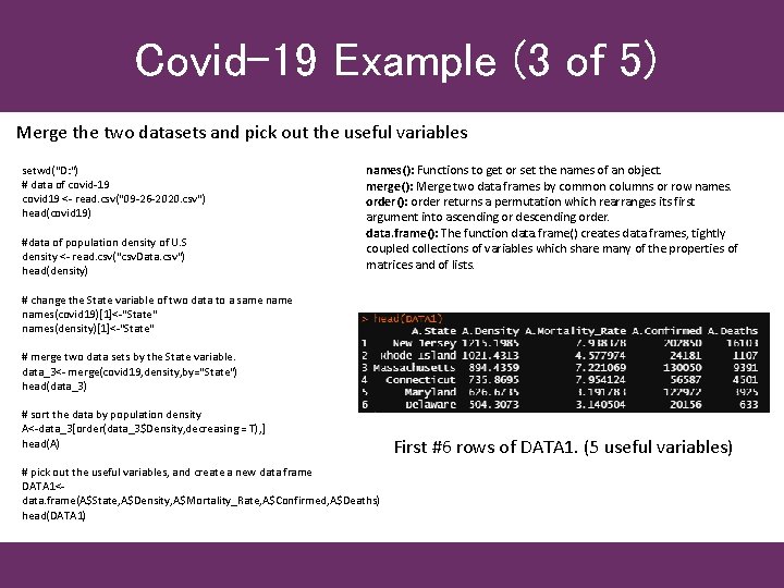
Covid-19 Example (3 of 5) Merge the two datasets and pick out the useful variables setwd("D: ") # data of covid-19 covid 19 <- read. csv("09 -26 -2020. csv") head(covid 19) #data of population density of U. S density <- read. csv("csv. Data. csv") head(density) names(): Functions to get or set the names of an object. merge(): Merge two data frames by common columns or row names. order(): order returns a permutation which rearranges its first argument into ascending or descending order. data. frame(): The function data. frame() creates data frames, tightly coupled collections of variables which share many of the properties of matrices and of lists. # change the State variable of two data to a same names(covid 19)[1]<-"State" names(density)[1]<-"State" # merge two data sets by the State variable. data_3<- merge(covid 19, density, by="State") head(data_3) # sort the data by population density A<-data_3[order(data_3$Density, decreasing = T), ] head(A) # pick out the useful variables, and create a new data frame DATA 1<data. frame(A$State, A$Density, A$Mortality_Rate, A$Confirmed, A$Deaths) head(DATA 1) First #6 rows of DATA 1. (5 useful variables)
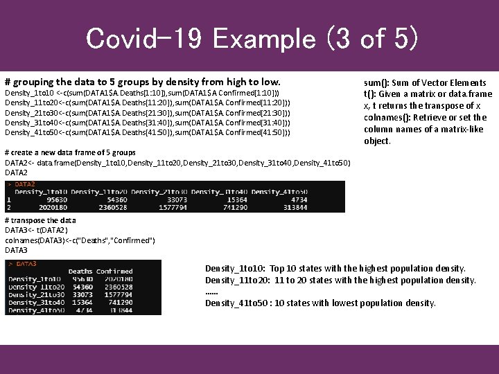
Covid-19 Example (3 of 5) # grouping the data to 5 groups by density from high to low. Density_1 to 10 <-c(sum(DATA 1$A. Deaths[1: 10]), sum(DATA 1$A. Confirmed[1: 10])) Density_11 to 20<-c(sum(DATA 1$A. Deaths[11: 20]), sum(DATA 1$A. Confirmed[11: 20])) Density_21 to 30<-c(sum(DATA 1$A. Deaths[21: 30]), sum(DATA 1$A. Confirmed[21: 30])) Density_31 to 40<-c(sum(DATA 1$A. Deaths[31: 40]), sum(DATA 1$A. Confirmed[31: 40])) Density_41 to 50<-c(sum(DATA 1$A. Deaths[41: 50]), sum(DATA 1$A. Confirmed[41: 50])) sum(): Sum of Vector Elements t(): Given a matrix or data. frame x, t returns the transpose of x colnames(): Retrieve or set the column names of a matrix-like object. # create a new data frame of 5 groups DATA 2<- data. frame(Density_1 to 10, Density_11 to 20, Density_21 to 30, Density_31 to 40, Density_41 to 50) DATA 2 # transpose the data DATA 3<- t(DATA 2) colnames(DATA 3)<-c("Deaths", "Confirmed") DATA 3 Density_1 to 10: Top 10 states with the highest population density. Density_11 to 20: 11 to 20 states with the highest population density. …… Density_41 to 50 : 10 states with lowest population density.
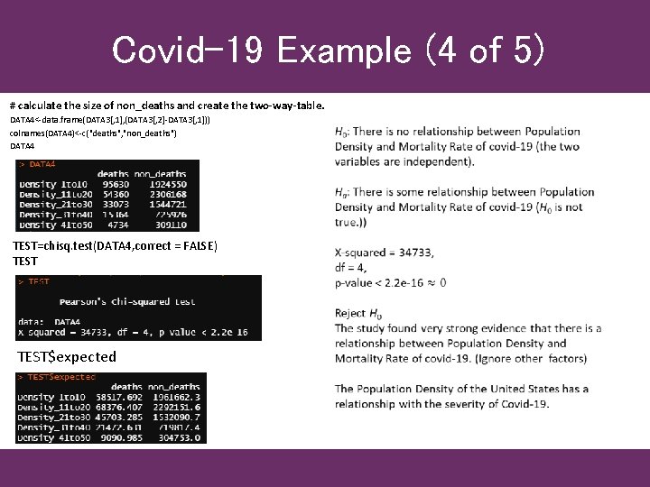
Covid-19 Example (4 of 5) # calculate the size of non_deaths and create the two-way-table. DATA 4<-data. frame(DATA 3[, 1], (DATA 3[, 2]-DATA 3[, 1])) colnames(DATA 4)<-c("deaths", "non_deaths") DATA 4 TEST=chisq. test(DATA 4, correct = FALSE) TEST$expected
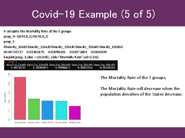
Covid-19 Example (5 of 5) # calculate the Mortality Rate of the 5 groups prop_3<-DATA 3[, 1]/DATA 3[, 2] prop_3 #Density_1 to 10 Density_11 to 20 Density_21 to 30 Density_31 to 40 Density_41 to 50 #0. 04733737 0. 02302875 0. 02096155 0. 02072603 0. 0150839 barplot(prop_3, ylim = c(0, 0. 05), ylab="Mortality Rate", col=c(2: 6)) The Mortality Rate of the 5 groups. The Mortality Rate will decrease when the population densities of the States decrease.
- Slides: 16