Chapter 21 ODEs Adaptive Methods and Stiff Systems

Chapter 21 ODEs: Adaptive Methods and Stiff Systems

Adaptive Runge Kutta Method Use small step size in high gradient region (abrupt change) automatic step size adjustment

Adaptive Runge Kutta Method z First approach: Step halving z Estimate local truncation error using two different step sizes z Solve each step twice, once as a full step and then as two half steps z Second approach: Embedded RK methods z (also called RK-Fehlberg methods) z Estimate local truncation error between two predictions using two different-order RK methods

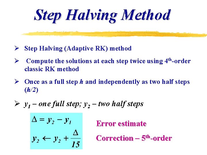
Step Halving Method Ø Step Halving (Adaptive RK) method Ø Compute the solutions at each step twice using 4 th-order classic RK method Ø Once as a full step h and independently as two half steps (h/2) Ø y 1 – one full step; y 2 – two half steps Error estimate Correction – 5 th-order

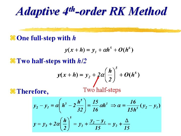
Adaptive th 4 -order RK Method z One full-step with h z Two half-steps with h/2 z Therefore, Two half-steps

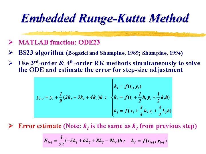
Embedded Runge-Kutta Method Ø MATLAB function: ODE 23 Ø BS 23 algorithm (Bogacki and Shampine, 1989; Shampine, 1994) Ø Use 3 rd-order & 4 th-order RK methods simultaneously to solve the ODE and estimate the error for step-size adjustment Ø Error estimate (Note: k 1 is the same as k 4 from previous step)

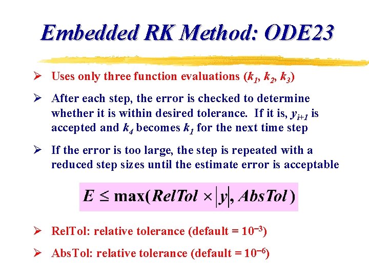
Embedded RK Method: ODE 23 Ø Uses only three function evaluations (k 1, k 2, k 3) Ø After each step, the error is checked to determine whether it is within desired tolerance. If it is, yi+1 is accepted and k 4 becomes k 1 for the next time step Ø If the error is too large, the step is repeated with a reduced step sizes until the estimate error is acceptable Ø Rel. Tol: relative tolerance (default = 10 3) Ø Abs. Tol: relative tolerance (default = 10 6)

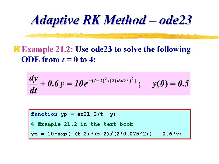
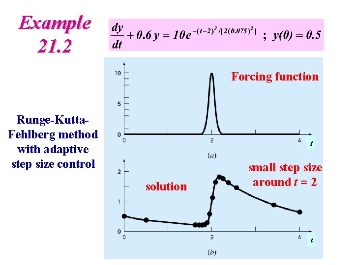
Adaptive RK Method – ode 23 z Example 21. 2: Use ode 23 to solve the following ODE from t = 0 to 4: function yp = ex 21_2(t, y) % Example 21. 2 in the text book yp = 10*exp(-(t-2)*(t-2)/(2*0. 075^2)) - 0. 6*y;

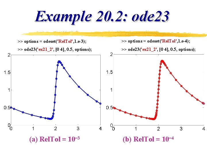
Example 20. 2: ode 23 >> options = odeset('Rel. Tol', 1. e-3); >> options = odeset('Rel. Tol', 1. e-4); >> ode 23('ex 21_2', [0 4], 0. 5, options); (a) Rel. Tol = 10 3 (b) Rel. Tol = 10 4

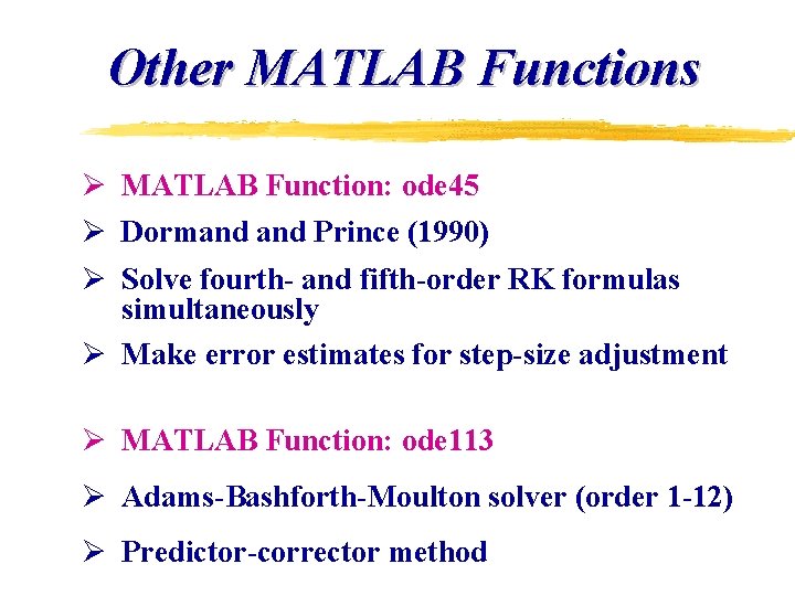
Other MATLAB Functions Ø MATLAB Function: ode 45 Ø Dormand Prince (1990) Ø Solve fourth- and fifth-order RK formulas simultaneously Ø Make error estimates for step-size adjustment Ø MATLAB Function: ode 113 Ø Adams-Bashforth-Moulton solver (order 1 -12) Ø Predictor-corrector method

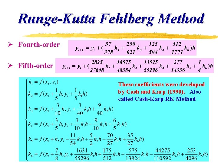
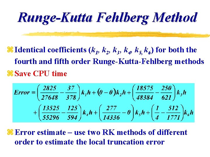
Runge-Kutta Fehlberg Method Ø Fourth-order Ø Fifth-order These coefficients were developed by Cash and Karp (1990). Also called Cash-Karp RK Method

Runge-Kutta Fehlberg Method z Identical coefficients (k 1, k 2, k 3, k 4, k 5, k 6) for both the fourth and fifth order Runge-Kutta-Fehlberg methods z Save CPU time z Error estimate – use two RK methods of different order to estimate the local truncation error

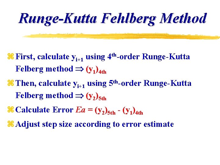
Runge-Kutta Fehlberg Method z First, calculate yi+1 using 4 th-order Runge-Kutta Felberg method (y 1)4 th z Then, calculate yi+1 using 5 th-order Runge-Kutta Felberg method (y 2)5 th z Calculate Error Ea = (y 2)5 th - (y 1)4 th z Adjust step size according to error estimate

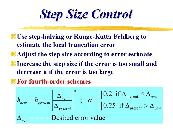
Step Size Control z Use step-halving or Runge-Kutta Fehlberg to estimate the local truncation error z Adjust the step size according to error estimate z Increase the step size if the error is too small and decrease it if the error is too large z For fourth-order schemes

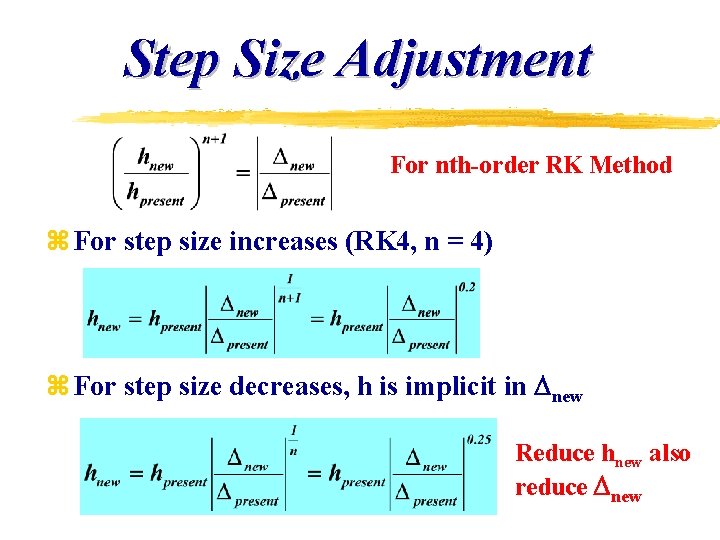
Step Size Adjustment For nth-order RK Method z For step size increases (RK 4, n = 4) z For step size decreases, h is implicit in new Reduce hnew also reduce new

Example 21. 2 Forcing function Runge-Kutta. Fehlberg method with adaptive step size control t solution small step size around t = 2 t

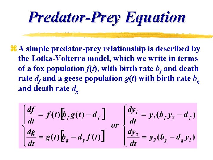
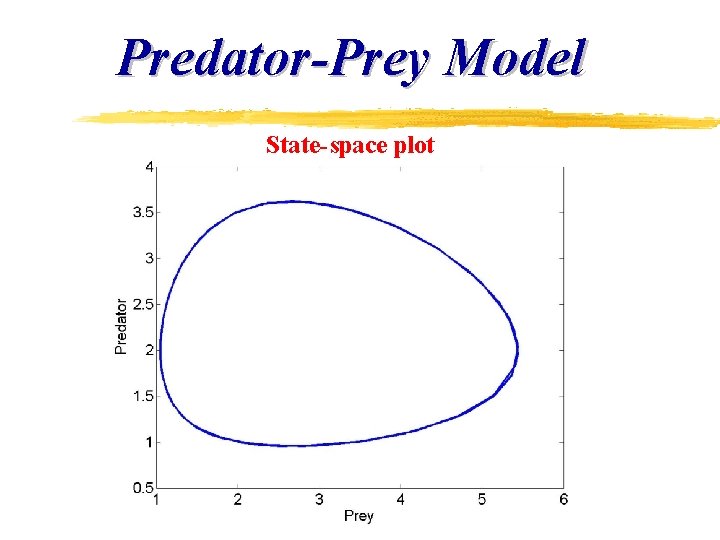
Predator-Prey Equation z A simple predator-prey relationship is described by the Lotka-Volterra model, which we write in terms of a fox population f(t), with birth rate bf and death rate df and a geese population g(t) with birth rate bg and death rate dg

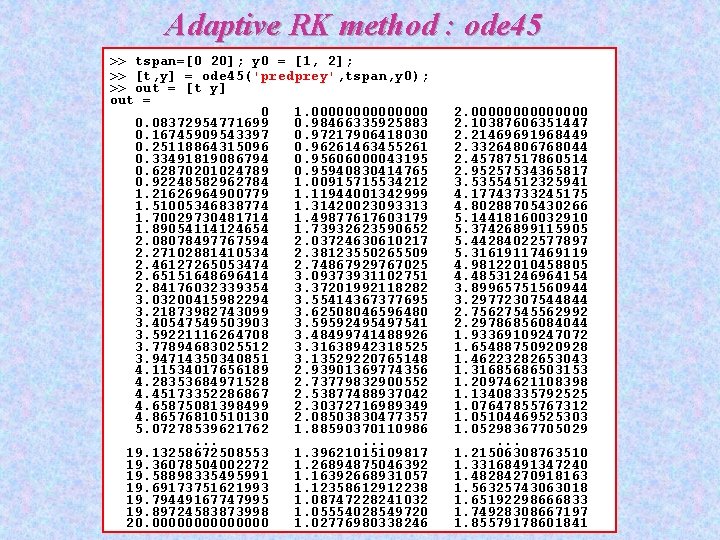
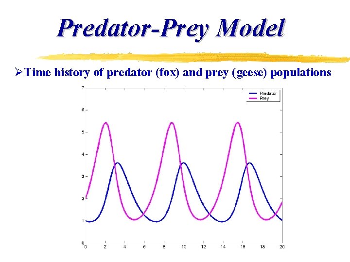
Predator-Prey Equation z Example: Given bf = 0. 3, df = 0. 8, bg = 1. 2, dg = 0. 6, find the populations of predators and preys as a function of time (t = 0 to 20) using ode 45. Predator Prey function yp = predprey(t, y) % Fox (Predator) population y 1(t), birth rate bf, death rate df % Geese (prey) poupulation y 2(t), birth rate bg, death rate dg bf = 0. 3; df = 0. 8; bg = 1. 2; dg = 0. 6; yp = [y(1)*(bf*y(2)-df); y(2)*(bg-dg*y(1))];

Adaptive RK method : ode 45 >> tspan=[0 20]; y 0 = [1, 2]; >> [t, y] = ode 45('predprey', tspan, y 0); >> out = [t y] out = 0 1. 0000000 0. 08372954771699 0. 98466335925883 0. 16745909543397 0. 97217906418030 0. 25118864315096 0. 96261463455261 0. 33491819086794 0. 95606000043195 0. 62870201024789 0. 95940830414765 0. 92248582962784 1. 00915715534212 1. 21626964900779 1. 11944001342999 1. 51005346838774 1. 31420023093313 1. 70029730481714 1. 49877617603179 1. 89054114124654 1. 73932623590652 2. 08078497767594 2. 03724630610217 2. 27102881410534 2. 38123550265509 2. 46127265053474 2. 74867929767025 2. 65151648696414 3. 09373931102751 2. 84176032339354 3. 37201992118282 3. 03200415982294 3. 55414367377695 3. 21873982743099 3. 62508046596480 3. 40547549503903 3. 59592495497541 3. 59221116264708 3. 48499741488926 3. 77894683025512 3. 31638942318525 3. 94714350340851 3. 13529220765148 4. 11534017656189 2. 93901369774356 4. 28353684971528 2. 73779832900552 4. 45173352286867 2. 53877488937042 4. 65875081398499 2. 30372716989349 4. 86576810510130 2. 08503830477357 5. 07278539621762 1. 88590370110986. . . 19. 13258672508553 1. 39621015109817 19. 36078504002272 1. 26894875046392 19. 58898335495991 1. 16392668931057 19. 69173751621993 1. 12358612912238 19. 79449167747995 1. 08747228241032 19. 89724583873998 1. 05554028549720 20. 0000000 1. 02776980338246 2. 0000000 2. 10387606351447 2. 21469691968449 2. 33264806768044 2. 45787517860514 2. 95257534365817 3. 53554512325941 4. 17743733245175 4. 80288705430266 5. 14418160032910 5. 37426899115905 5. 44284022577897 5. 31619117469119 4. 98122010458805 4. 48531246964154 3. 89965751560944 3. 29772307544844 2. 75627545562992 2. 29786856084044 1. 93369109247072 1. 65488750920928 1. 46223282653043 1. 31685686503153 1. 20974621108398 1. 13408335792525 1. 07647855767312 1. 05104469525303 1. 05298367705029. . . 1. 21506308763510 1. 33168491347240 1. 48284270918163 1. 56325743063018 1. 65192298666833 1. 74928308667197 1. 85579178601841

Predator-Prey Model ØTime history of predator (fox) and prey (geese) populations

Predator-Prey Model State-space plot

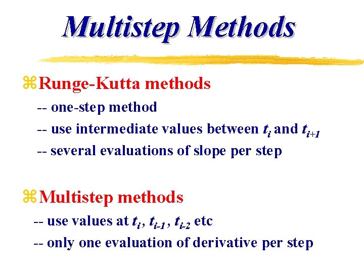
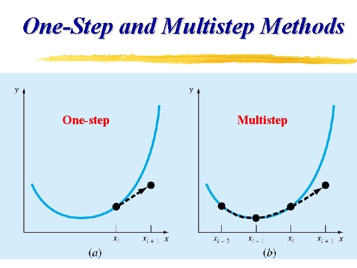
Multistep Methods z. Runge-Kutta methods -- one-step method -- use intermediate values between ti and ti+1 -- several evaluations of slope per step z. Multistep methods -- use values at ti , ti-1 , ti-2 etc -- only one evaluation of derivative per step

One-Step and Multistep Methods One-step Multistep

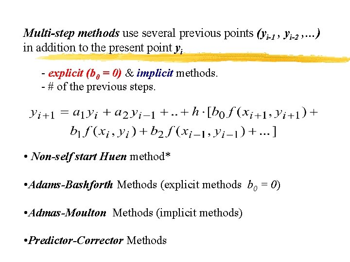
Multi-step methods use several previous points (yi-1 , yi-2 , …) in addition to the present point yi - explicit (b 0 = 0) & implicit methods. - # of the previous steps. • Non-self start Huen method* • Adams-Bashforth Methods (explicit methods b 0 = 0) • Admas-Moulton Methods (implicit methods) • Predictor-Corrector Methods

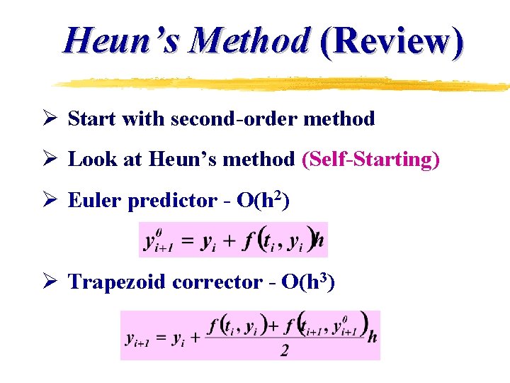
Heun’s Method (Review) Ø Start with second-order method Ø Look at Heun’s method (Self-Starting) Ø Euler predictor - O(h 2) Ø Trapezoid corrector - O(h 3)

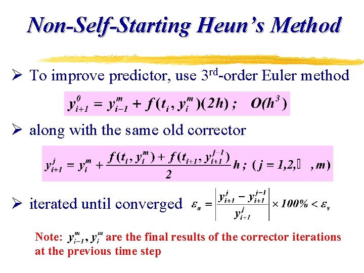
Non-Self-Starting Heun’s Method Ø To improve predictor, use 3 rd-order Euler method Ø along with the same old corrector Ø iterated until converged Note: are the final results of the corrector iterations at the previous time step

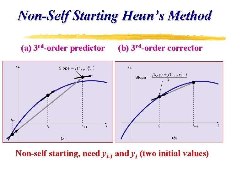
Non-Self Starting Heun’s Method (a) 3 rd-order predictor (b) 3 rd-order corrector Non-self starting, need yi-1 and yi (two initial values)

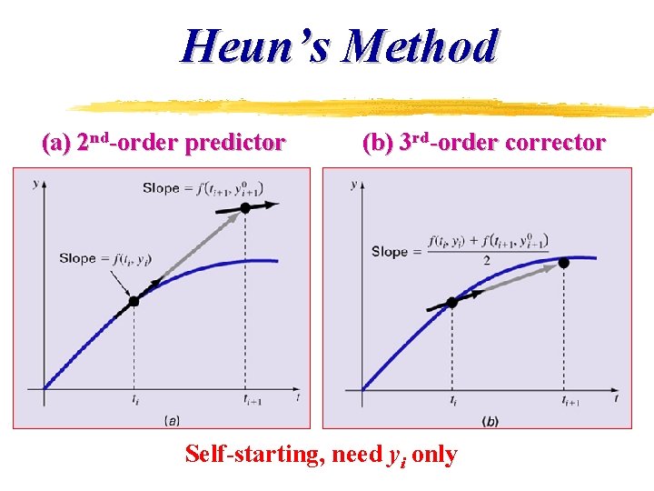
Heun’s Method (a) 2 nd-order predictor (b) 3 rd-order corrector Self-starting, need yi only

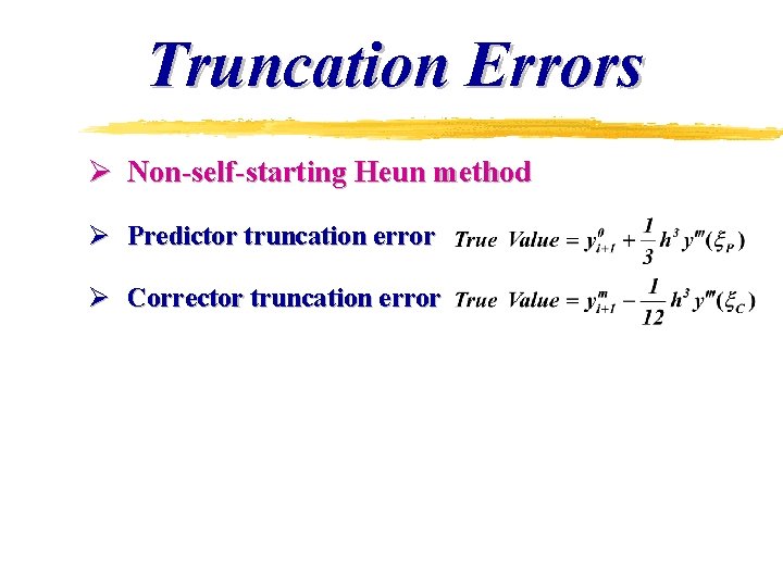
Truncation Errors Ø Non-self-starting Heun method Ø Predictor truncation error Ø Corrector truncation error

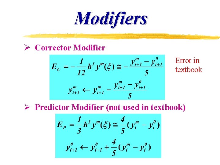
Modifiers Ø Corrector Modifier Error in textbook Ø Predictor Modifier (not used in textbook)

Non-Self Starting Heun’s Method So the sequence is q Predict q Adjust prediction* q Correct q Converged? q If not, correct again

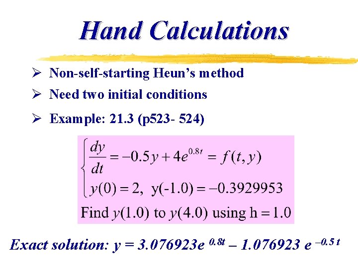
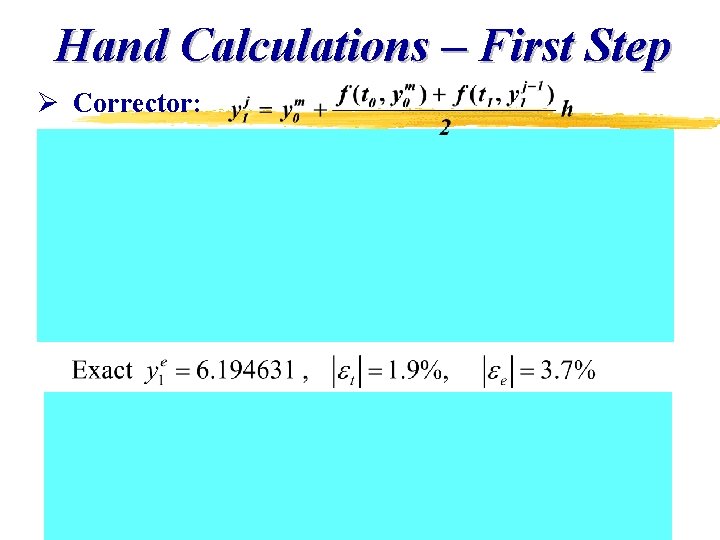
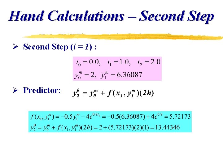
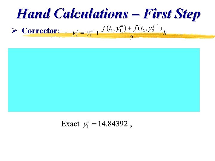
Hand Calculations Ø Non-self-starting Heun’s method Ø Need two initial conditions Ø Example: 21. 3 (p 523 - 524) Exact solution: y = 3. 076923 e 0. 8 t – 1. 076923 e – 0. 5 t

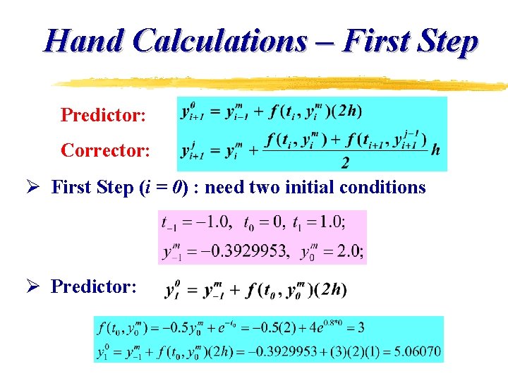
Hand Calculations – First Step Predictor: Corrector: Ø First Step (i = 0) : need two initial conditions Ø Predictor:

Hand Calculations – First Step Ø Corrector:

Hand Calculations – Second Step Ø Second Step (i = 1) : Ø Predictor:

Hand Calculations – First Step Ø Corrector:

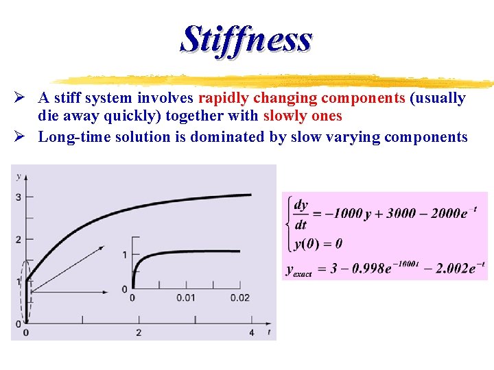
Stiffness Ø A stiff system involves rapidly changing components (usually die away quickly) together with slowly ones Ø Long-time solution is dominated by slow varying components

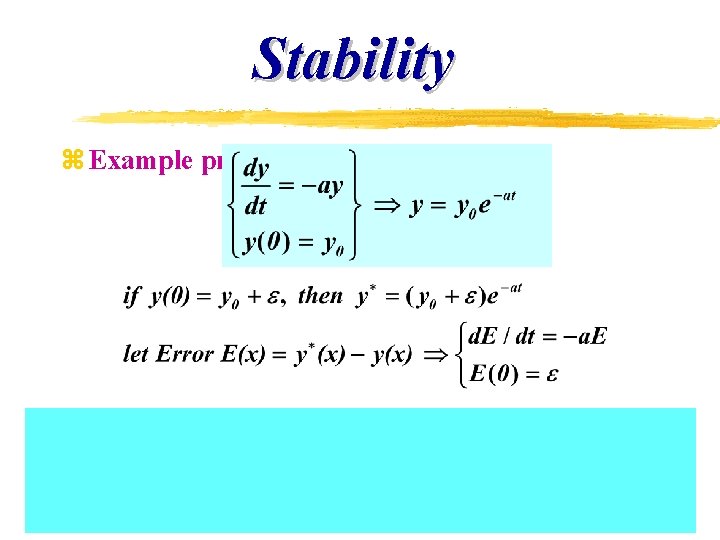
Numerical Stability z Amplification or decay of numerical errors z A numerical method is stable if error incurred at one stage of the process do not tend to magnify at later stages z Ill-conditioned differential equation -- numerical errors will be magnified regardless of numerical method z Stiff differential equation -- require extremely small step size to achieve accurate results

Stability z Example problem

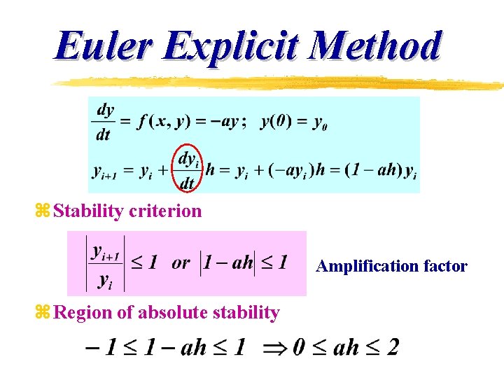
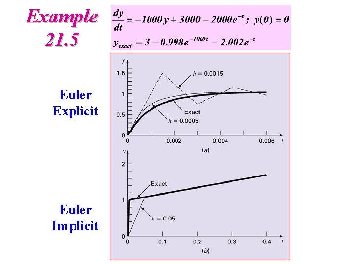
Euler Explicit Method z Stability criterion Amplification factor z Region of absolute stability

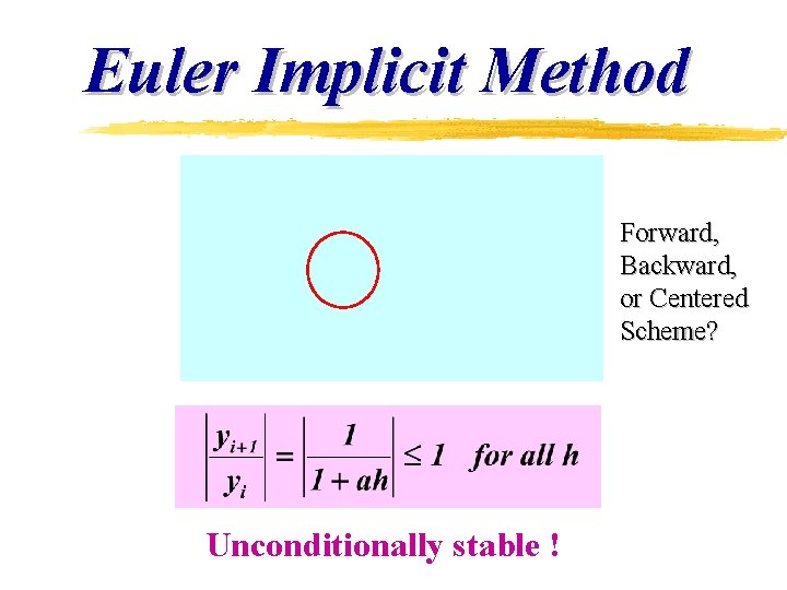
Euler Implicit Method Forward, Backward, or Centered Scheme? Unconditionally stable !

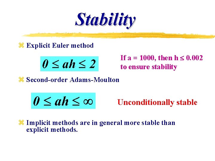
Stability z Explicit Euler method If a = 1000, then h 0. 002 to ensure stability z Second-order Adams-Moulton Unconditionally stable z Implicit methods are in general more stable than explicit methods.

Example 21. 5 Euler Explicit Euler Implicit

MATLAB Functions for Stiff Systems z ode 15 s – based on Gear backward differentiation for stiff problems of low to medium accuracy z ode 23 s – based on modified Rosenbrock formula z ode 23 t – trapezoidal rule with a free interpolant for moderately stiff problems without numerical damping z ode 23 tb – implicit Runge-Kutta formula for more explanation please see page 529

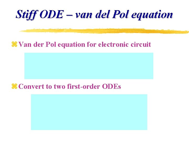
Stiff ODE – van del Pol equation z Van der Pol equation for electronic circuit z Convert to two first-order ODEs

Stiff ODE – van del Pol equation z M-file for van del Pol equation function yp = vanderpol(t, y, mu) % van der Pol equation for electronic circuit % d^2 y 1/dt^2 - mu*(1 -y 1^2) * dy 1/dt + y 1 = 0 % initial conditions, y 1(0) = dy 1/dt = 1 % convert to two first-order ODEs % The solution becomes progressively stiffer % as mu gets large yp = [y(2); mu*(1 -y(1)^2)*y(2)-y(1)];

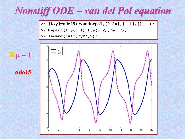
Nonstiff ODE – van del Pol equation >> [t, y]=ode 45(@vanderpol, [0 20], [1 1], [], 1); >> H=plot(t, y(: , 1), t, y(: , 2), 'm--'); >> legend('y 1', 'y 2', 2); z = 1 ode 45

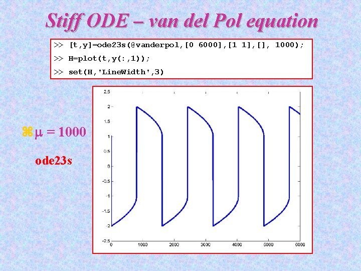
Stiff ODE – van del Pol equation >> [t, y]=ode 23 s(@vanderpol, [0 6000], [1 1], [], 1000); >> H=plot(t, y(: , 1)); >> set(H, 'Line. Width', 3) z = 1000 ode 23 s

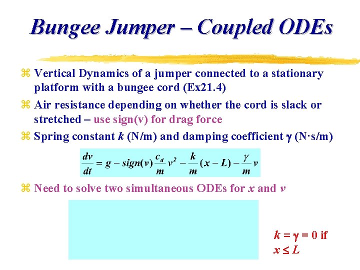
Bungee Jumper – Coupled ODEs z Vertical Dynamics of a jumper connected to a stationary platform with a bungee cord (Ex 21. 4) z Air resistance depending on whether the cord is slack or stretched – use sign(v) for drag force z Spring constant k (N/m) and damping coefficient (N·s/m) z Need to solve two simultaneous ODEs for x and v k = = 0 if x L

Non-stiff ODEs: Bungee Jumper z Use ode 45 for non-stiff ODEs to solve for the distance and velocity of a bungee jumper function dydt = bungee(t, y, L, cd, m, k, gamma) g = 9. 81; cord = 0; if y(1) > L % determine if the cord exerts a force cord = k/m * (y(1)-L) + gamma/m * y(2); end dydt = [y(2); g - sign(y(2)) * cd/m*y(2)^2 - cord];

>> [t, y] = ode 45(@bungee, [0 50], [0 0], [], 30, 0. 25, 68. 1, 40, 8); >> h 1 = plot(t, -y(: , 1), t, y(: , 2), 'm--'); >> h 2 = legend('x (m)', 'v(m/s)'); >> set(h 1, 'Line. Width', 3); set(h 2, 'Font. Size', 12); Bungee jumper velocity Bungee jumper distance

CVEN 302 -501 Homework No. 14 z. Chapter 21 z Prob. 21. 3 (30) (Hand Calculation) 21. 5 (30) z Prob. 21. 8 (40) (using MATLAB program except for part a)) z Due 12/02/08 before 5: 00 pm