Chapter 20 The ISLM Model Copyright 2010 Pearson

Chapter 20 • The ISLM Model Copyright © 2010 Pearson Education. All rights reserved.

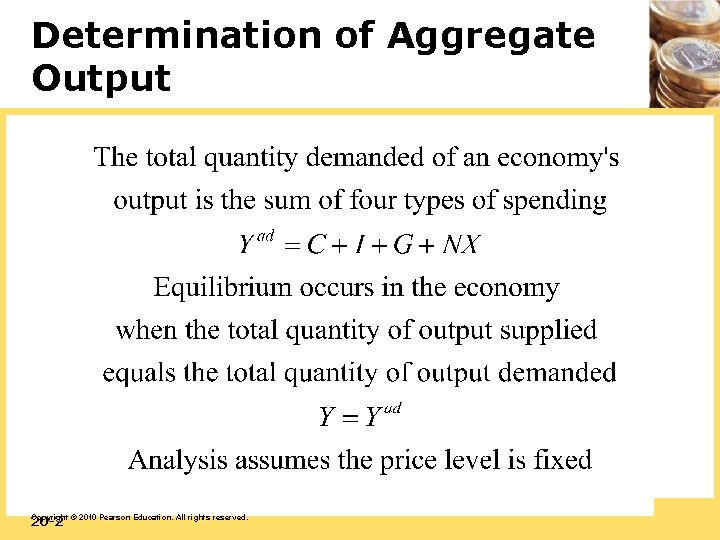
Determination of Aggregate Output 20 -2 Copyright © 2010 Pearson Education. All rights reserved.

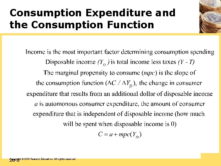
Consumption Expenditure and the Consumption Function 20 -3 Copyright © 2010 Pearson Education. All rights reserved.

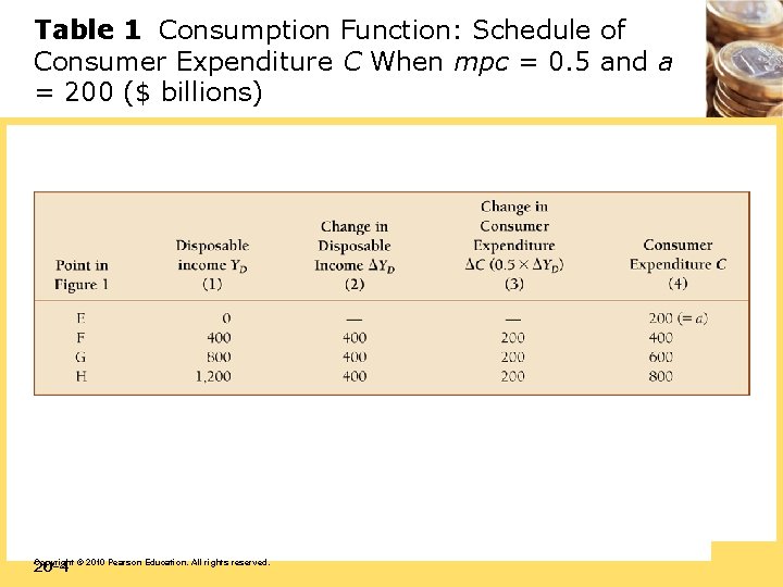
Table 1 Consumption Function: Schedule of Consumer Expenditure C When mpc = 0. 5 and a = 200 ($ billions) 20 -4 Copyright © 2010 Pearson Education. All rights reserved.

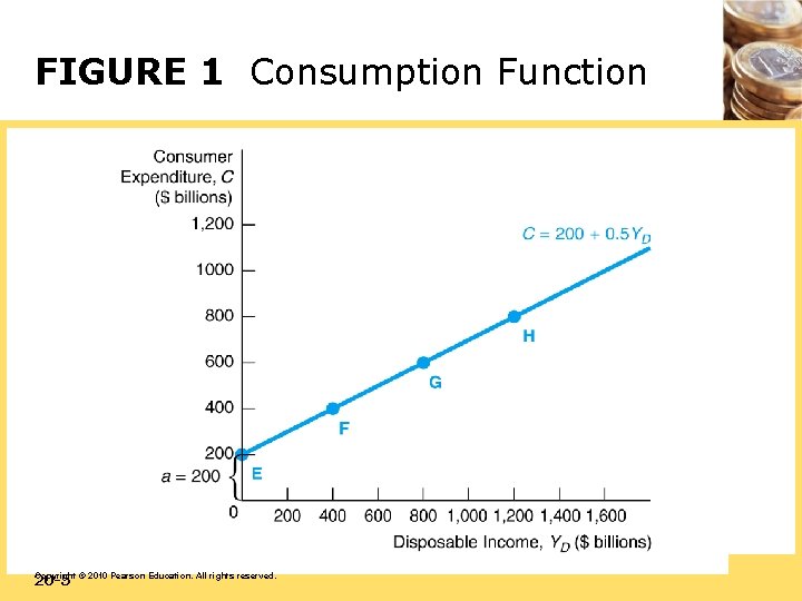
FIGURE 1 Consumption Function 20 -5 Copyright © 2010 Pearson Education. All rights reserved.

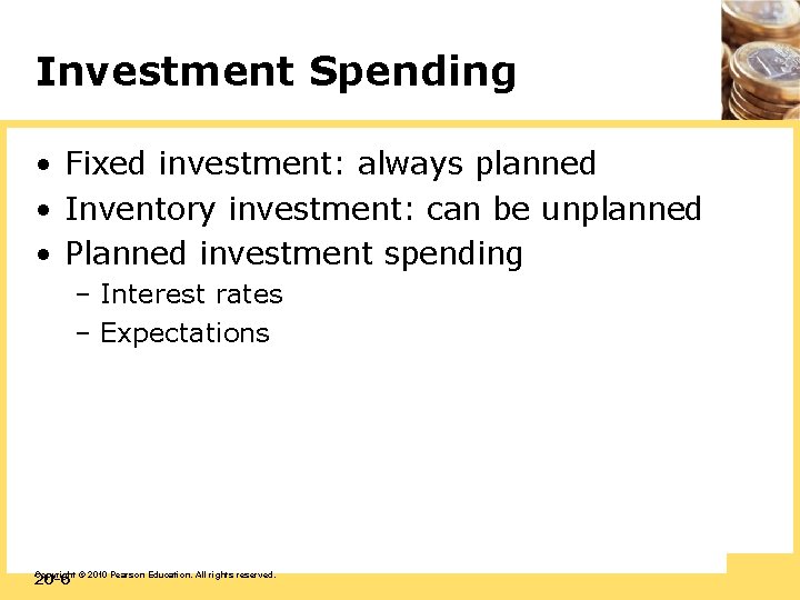
Investment Spending • Fixed investment: always planned • Inventory investment: can be unplanned • Planned investment spending – Interest rates – Expectations 20 -6 Copyright © 2010 Pearson Education. All rights reserved.

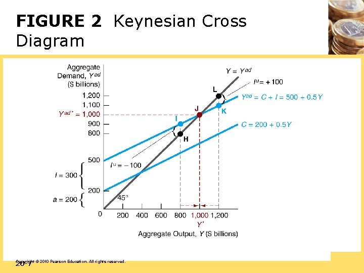
FIGURE 2 Keynesian Cross Diagram 20 -7 Copyright © 2010 Pearson Education. All rights reserved.

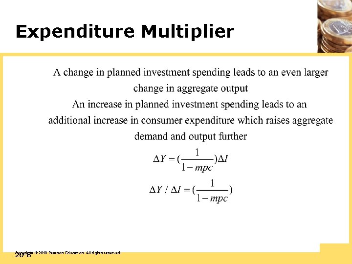
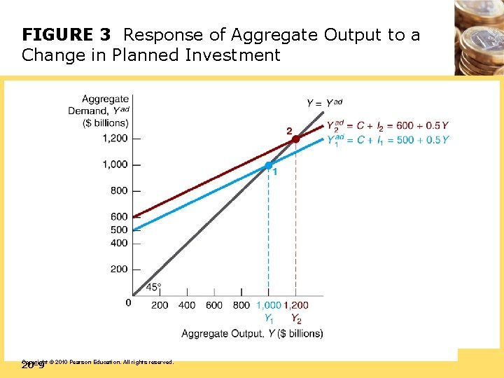
Expenditure Multiplier 20 -8 Copyright © 2010 Pearson Education. All rights reserved.

FIGURE 3 Response of Aggregate Output to a Change in Planned Investment 20 -9 Copyright © 2010 Pearson Education. All rights reserved.

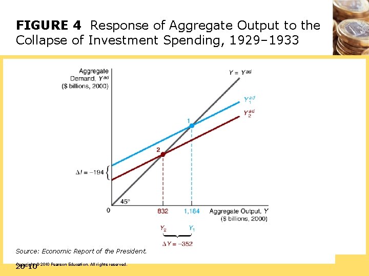
FIGURE 4 Response of Aggregate Output to the Collapse of Investment Spending, 1929– 1933 Source: Economic Report of the President. 20 -10 Copyright © 2010 Pearson Education. All rights reserved.

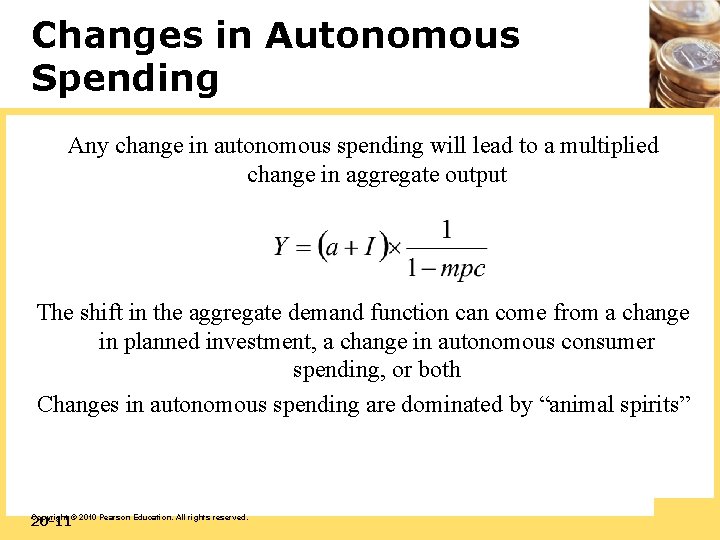
Changes in Autonomous Spending Any change in autonomous spending will lead to a multiplied change in aggregate output The shift in the aggregate demand function can come from a change in planned investment, a change in autonomous consumer spending, or both Changes in autonomous spending are dominated by “animal spirits” 20 -11 Copyright © 2010 Pearson Education. All rights reserved.

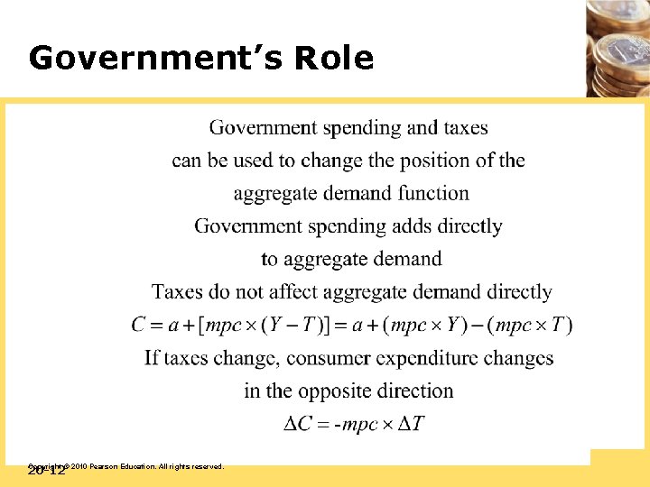
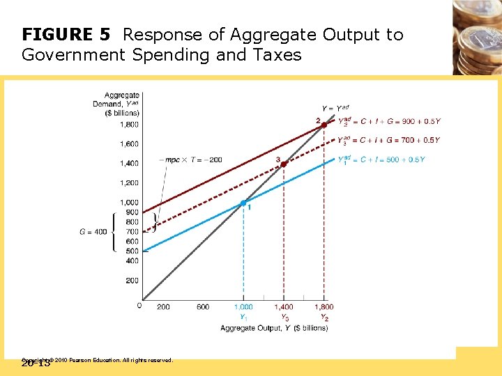
Government’s Role 20 -12 Copyright © 2010 Pearson Education. All rights reserved.

FIGURE 5 Response of Aggregate Output to Government Spending and Taxes 20 -13 Copyright © 2010 Pearson Education. All rights reserved.

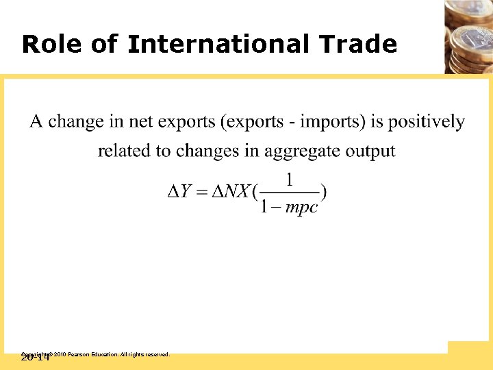
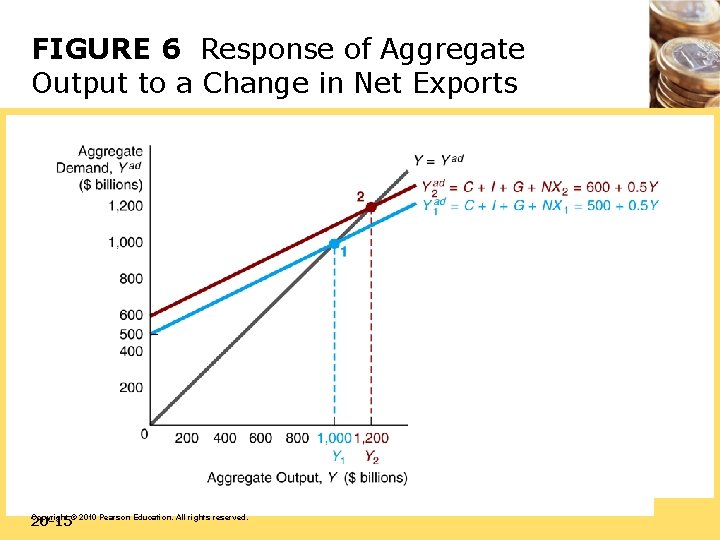
Role of International Trade 20 -14 Copyright © 2010 Pearson Education. All rights reserved.

FIGURE 6 Response of Aggregate Output to a Change in Net Exports 20 -15 Copyright © 2010 Pearson Education. All rights reserved.

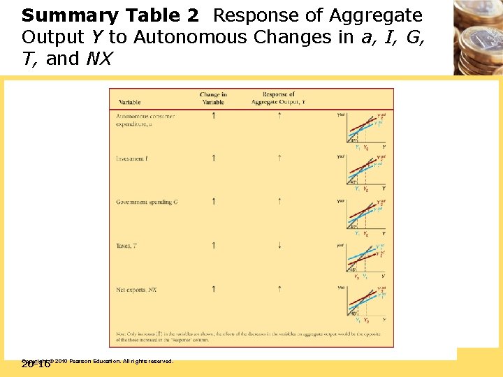
Summary Table 2 Response of Aggregate Output Y to Autonomous Changes in a, I, G, T, and NX 20 -16 Copyright © 2010 Pearson Education. All rights reserved.

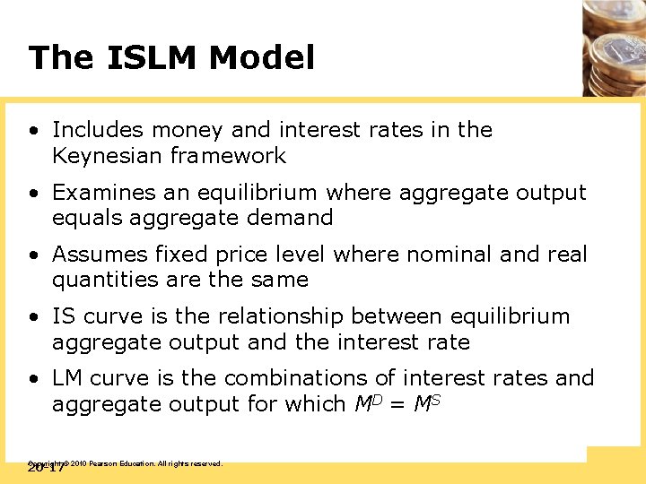
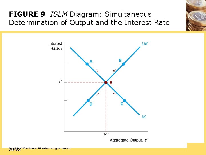
The ISLM Model • Includes money and interest rates in the Keynesian framework • Examines an equilibrium where aggregate output equals aggregate demand • Assumes fixed price level where nominal and real quantities are the same • IS curve is the relationship between equilibrium aggregate output and the interest rate • LM curve is the combinations of interest rates and aggregate output for which MD = MS 20 -17 Copyright © 2010 Pearson Education. All rights reserved.

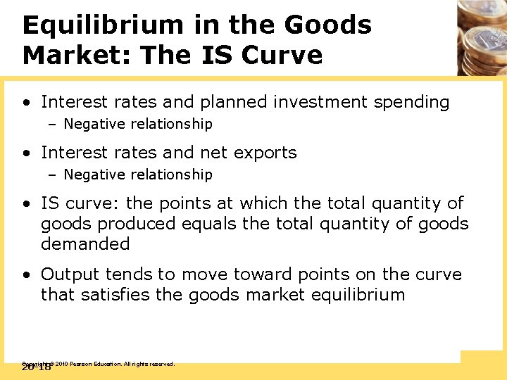
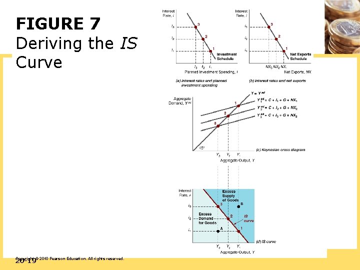
Equilibrium in the Goods Market: The IS Curve • Interest rates and planned investment spending – Negative relationship • Interest rates and net exports – Negative relationship • IS curve: the points at which the total quantity of goods produced equals the total quantity of goods demanded • Output tends to move toward points on the curve that satisfies the goods market equilibrium 20 -18 Copyright © 2010 Pearson Education. All rights reserved.

FIGURE 7 Deriving the IS Curve 20 -19 Copyright © 2010 Pearson Education. All rights reserved.

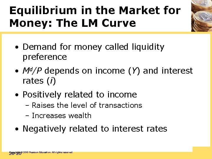
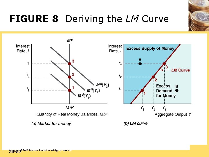
Equilibrium in the Market for Money: The LM Curve • Demand for money called liquidity preference • Md/P depends on income (Y) and interest rates (i) • Positively related to income – Raises the level of transactions – Increases wealth • Negatively related to interest rates 20 -20 Copyright © 2010 Pearson Education. All rights reserved.

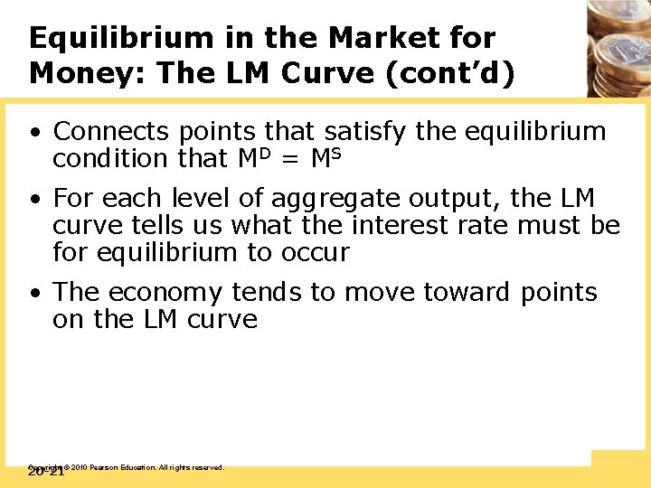
Equilibrium in the Market for Money: The LM Curve (cont’d) • Connects points that satisfy the equilibrium condition that MD = MS • For each level of aggregate output, the LM curve tells us what the interest rate must be for equilibrium to occur • The economy tends to move toward points on the LM curve 20 -21 Copyright © 2010 Pearson Education. All rights reserved.

FIGURE 8 Deriving the LM Curve 20 -22 Copyright © 2010 Pearson Education. All rights reserved.

FIGURE 9 ISLM Diagram: Simultaneous Determination of Output and the Interest Rate 20 -23 Copyright © 2010 Pearson Education. All rights reserved.