Chapter 20 Part 2 Computational Lexical Semantics Acknowledgements

Chapter 20 Part 2 Computational Lexical Semantics Acknowledgements: these slides include material from Rada Mihalcea, Ray Mooney, Katrin Erk, and Ani Nenkova 1

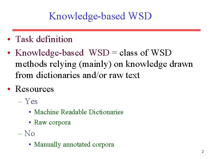
Knowledge-based WSD • Task definition • Knowledge-based WSD = class of WSD methods relying (mainly) on knowledge drawn from dictionaries and/or raw text • Resources – Yes • Machine Readable Dictionaries • Raw corpora – No • Manually annotated corpora 2

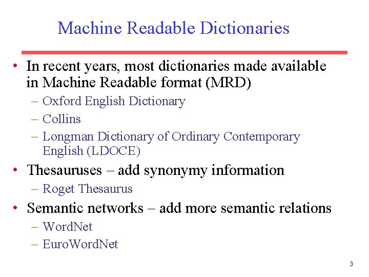
Machine Readable Dictionaries • In recent years, most dictionaries made available in Machine Readable format (MRD) – Oxford English Dictionary – Collins – Longman Dictionary of Ordinary Contemporary English (LDOCE) • Thesauruses – add synonymy information – Roget Thesaurus • Semantic networks – add more semantic relations – Word. Net – Euro. Word. Net 3

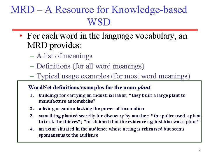
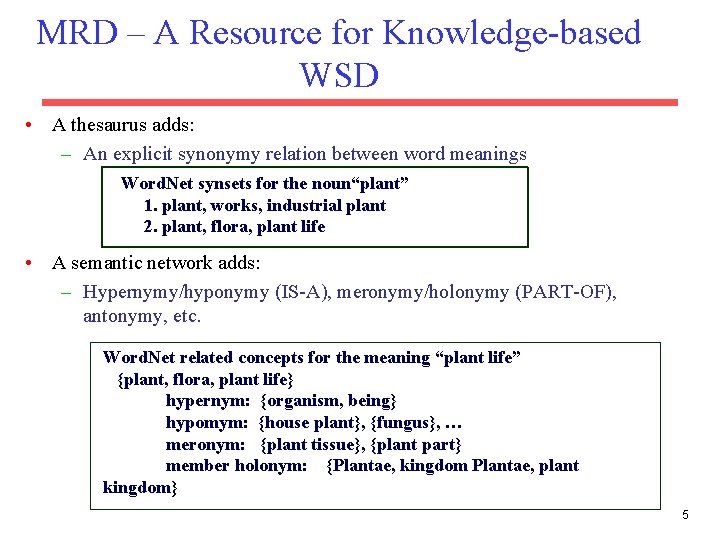
MRD – A Resource for Knowledge-based WSD • For each word in the language vocabulary, an MRD provides: – A list of meanings – Definitions (for all word meanings) – Typical usage examples (for most word meanings) Word. Net definitions/examples for the noun plant 1. buildings for carrying on industrial labor; "they built a large plant to manufacture automobiles” 2. a living organism lacking the power of locomotion 3. something planted secretly for discovery by another; "the police used a plant to trick the thieves"; "he claimed that the evidence against him was a plant" 4. an actor situated in the audience whose acting is rehearsed but seems spontaneous to the audience 4

MRD – A Resource for Knowledge-based WSD • A thesaurus adds: – An explicit synonymy relation between word meanings Word. Net synsets for the noun“plant” 1. plant, works, industrial plant 2. plant, flora, plant life • A semantic network adds: – Hypernymy/hyponymy (IS-A), meronymy/holonymy (PART-OF), antonymy, etc. Word. Net related concepts for the meaning “plant life” {plant, flora, plant life} hypernym: {organism, being} hypomym: {house plant}, {fungus}, … meronym: {plant tissue}, {plant part} member holonym: {Plantae, kingdom Plantae, plant kingdom} 5

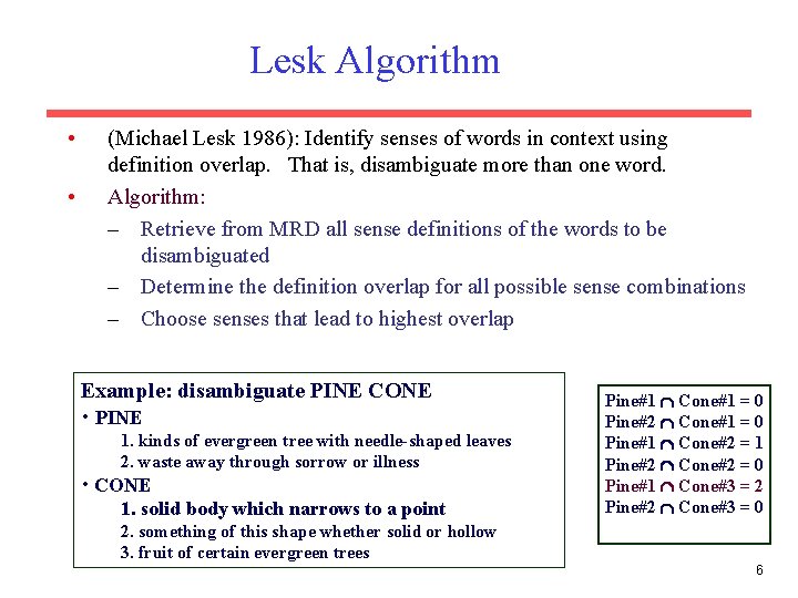
Lesk Algorithm • • (Michael Lesk 1986): Identify senses of words in context using definition overlap. That is, disambiguate more than one word. Algorithm: – Retrieve from MRD all sense definitions of the words to be disambiguated – Determine the definition overlap for all possible sense combinations – Choose senses that lead to highest overlap Example: disambiguate PINE CONE • PINE 1. kinds of evergreen tree with needle-shaped leaves 2. waste away through sorrow or illness • CONE 1. solid body which narrows to a point Pine#1 Cone#1 = 0 Pine#2 Cone#1 = 0 Pine#1 Cone#2 = 1 Pine#2 Cone#2 = 0 Pine#1 Cone#3 = 2 Pine#2 Cone#3 = 0 2. something of this shape whether solid or hollow 3. fruit of certain evergreen trees 6

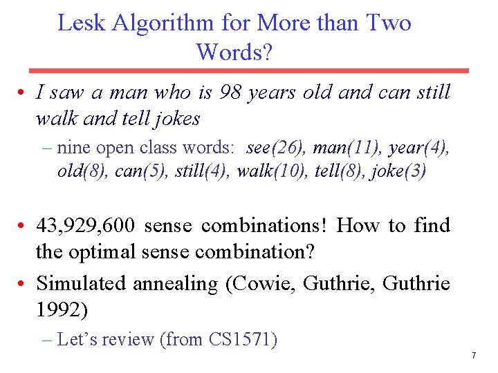
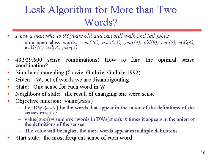
Lesk Algorithm for More than Two Words? • I saw a man who is 98 years old and can still walk and tell jokes – nine open class words: see(26), man(11), year(4), old(8), can(5), still(4), walk(10), tell(8), joke(3) • 43, 929, 600 sense combinations! How to find the optimal sense combination? • Simulated annealing (Cowie, Guthrie 1992) – Let’s review (from CS 1571) 7

Search Types – Backtracking state-space search – Local Search and Optimization – Constraint satisfaction search – Adversarial search • 8

Local Search • Use a single current state and move only to neighbors. • Use little space • Can find reasonable solutions in large or infinite (continuous) state spaces for which the other algorithms are not suitable • 9

Optimization • Local search is often suitable for optimization problems. Search for best state by optimizing an objective function. • 10

Visualization • States are laid out in a landscape • Height corresponds to the objective function value • Move around the landscape to find the highest (or lowest) peak • Only keep track of the current states and immediate neighbors • 11

Simulated Annealing • Based on a metallurgical metaphor – Start with a temperature set very high and slowly reduce it. • 12

Simulated Annealing • Annealing: harden metals and glass by heating them to a high temperature and then gradually cooling them • At the start, make lots of moves and then gradually slow down • 13

Simulated Annealing • More formally… – Generate a random new neighbor from current state. – If it’s better take it. – If it’s worse then take it with some probability proportional to the temperature and the delta between the new and old states. • 14

Simulated annealing • Probability of a move decreases with the amount ΔE by which the evaluation is worsened • A second parameter T is also used to determine the probability: high T allows more worse moves, T close to zero results in few or no bad moves • Schedule input determines the value of T as a function of the completed cycles • 15

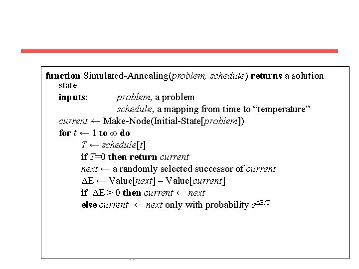
function Simulated-Annealing(problem, schedule) returns a solution state inputs: problem, a problem schedule, a mapping from time to “temperature” current ← Make-Node(Initial-State[problem]) for t ← 1 to ∞ do T ← schedule[t] if T=0 then return current next ← a randomly selected successor of current ΔE ← Value[next] – Value[current] if ΔE > 0 then current ← next else current ← next only with probability eΔE/T • 16

Intuitions • the algorithm wanders around during the early parts of the search, hopefully toward a good general region of the state space • Toward the end, the algorithm does a more focused search, making few bad moves • 17

Lesk Algorithm for More than Two Words? • I saw a man who is 98 years old and can still walk and tell jokes – nine open class words: see(26), man(11), year(4), old(8), can(5), still(4), walk(10), tell(8), joke(3) • 43, 929, 600 sense combinations! How to find the optimal sense combination? • Simulated annealing (Cowie, Guthrie 1992) • Given: W, set of words we are disambiguating • State: One sense for each word in W • Neighbors of state: the result of changing one word sense • Objective function: value(state) – Let DWs(state) be the words that appear in the union of the definitions of the senses in state; – value(state) = sum over words in DWs(state): # times it appears in the union of the definitions of the senses – The value will be higher, the more words appear in multiple definitions. • Start state: the most frequent sense of each word 18

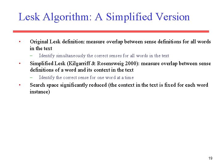
Lesk Algorithm: A Simplified Version • Original Lesk definition: measure overlap between sense definitions for all words in the text – • Simplified Lesk (Kilgarriff & Rosensweig 2000): measure overlap between sense definitions of a word and its context in the text – • Identify simultaneously the correct senses for all words in the text Identify the correct sense for one word at a time Search space significantly reduced (the context in the text is fixed for each word instance) 19

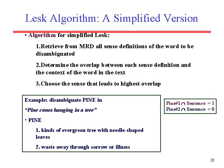
Lesk Algorithm: A Simplified Version • Algorithm for simplified Lesk: 1. Retrieve from MRD all sense definitions of the word to be disambiguated 2. Determine the overlap between each sense definition and the context of the word in the text 3. Choose the sense that leads to highest overlap Example: disambiguate PINE in “Pine cones hanging in a tree” Pine#1 Sentence = 1 Pine#2 Sentence = 0 • PINE 1. kinds of evergreen tree with needle-shaped leaves 2. waste away through sorrow or illness 20

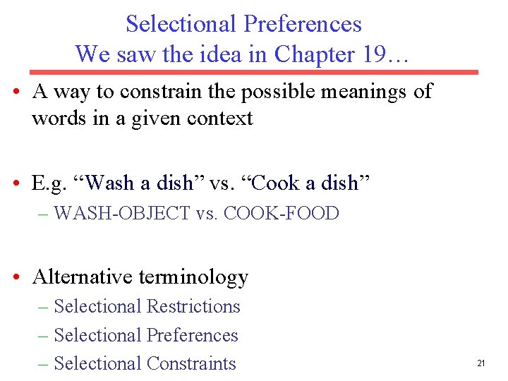
Selectional Preferences We saw the idea in Chapter 19… • A way to constrain the possible meanings of words in a given context • E. g. “Wash a dish” vs. “Cook a dish” – WASH-OBJECT vs. COOK-FOOD • Alternative terminology – Selectional Restrictions – Selectional Preferences – Selectional Constraints 21

Acquiring Selectional Preferences • From raw corpora – Frequency counts – Information theory measures 22

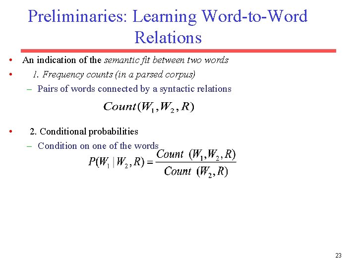
Preliminaries: Learning Word-to-Word Relations • An indication of the semantic fit between two words • 1. Frequency counts (in a parsed corpus) – Pairs of words connected by a syntactic relations • 2. Conditional probabilities – Condition on one of the words 23

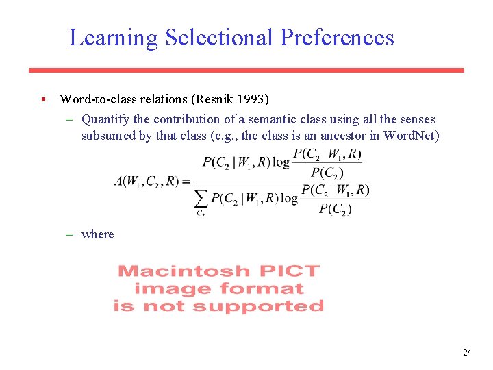
Learning Selectional Preferences • Word-to-class relations (Resnik 1993) – Quantify the contribution of a semantic class using all the senses subsumed by that class (e. g. , the class is an ancestor in Word. Net) – where 24

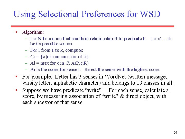
Using Selectional Preferences for WSD • Algorithm: – Let N be a noun that stands in relationship R to predicate P. Let s 1…sk be its possible senses. – For i from 1 to k, compute: – Ci = {c |c is an ancestor of si} – Ai = max for c in Ci A(P, c, R) – Ai is the score for sense i. Select the sense with the highest score. • For example: Letter has 3 senses in Word. Net (written message; varsity letter; alphabetic character) and belongs to 19 classes in all. • Suppose we have predicate “write”. For each sense, calculate a score, by measuring association of “write” & direct object, with each ancestor of that sense. 25

Similarity Metrics • Similarity metrics are useful not just for word sense disambiguation, but also for: – Finding topics of documents – Representing word meanings, not with respect to a fixed sense inventory • We will start with vector space models, and then look at dictionary based methods 26

Document Similarity • The ideas in vector space models are applied most widely to finding similar documents. • So, let’s think about documents, and then we will return to words 27

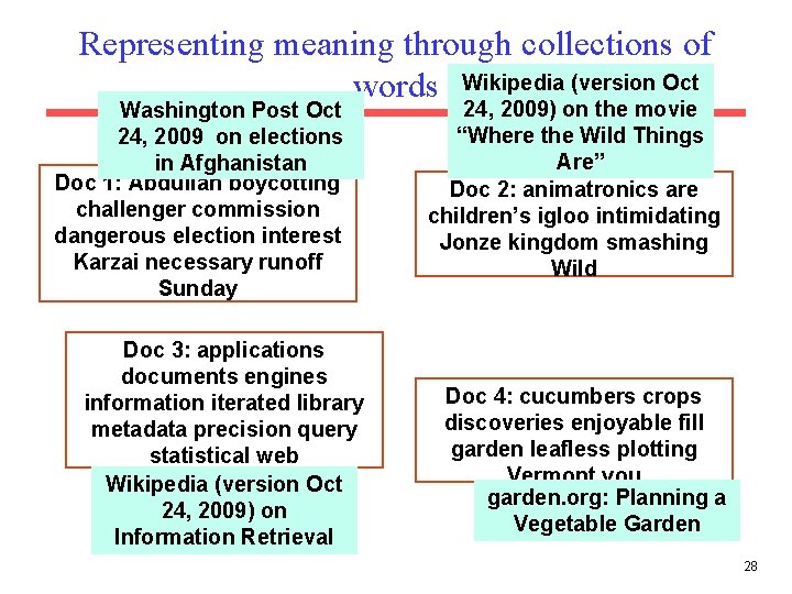
Representing meaning through collections of words Wikipedia (version Oct Washington Post Oct 24, 2009 on elections in Afghanistan Doc 1: Abdullah boycotting challenger commission dangerous election interest Karzai necessary runoff Sunday Doc 3: applications documents engines information iterated library metadata precision query statistical web Wikipedia (version Oct 24, 2009) on Information Retrieval 24, 2009) on the movie “Where the Wild Things Are” Doc 2: animatronics are children’s igloo intimidating Jonze kingdom smashing Wild Doc 4: cucumbers crops discoveries enjoyable fill garden leafless plotting Vermont you garden. org: Planning a Vegetable Garden 28

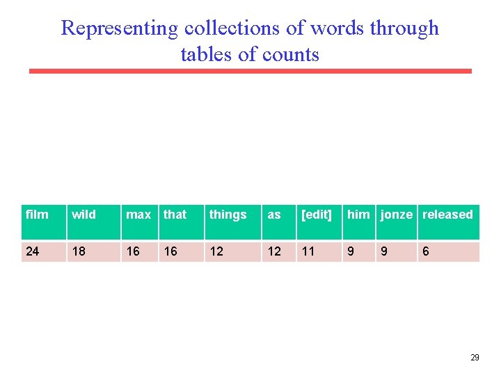
Representing collections of words through tables of counts film wild max that things as [edit] him jonze released 24 18 16 16 12 12 11 9 9 6 29

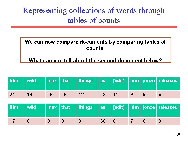
Representing collections of words through tables of counts We can now compare documents by comparing tables of counts. What can you tell about the second document below? film wild max that things as [edit] him jonze released 24 18 16 16 12 12 11 9 film wild max that things as [edit] him jonze released 17 0 0 9 0 36 8 7 9 0 6 3 30

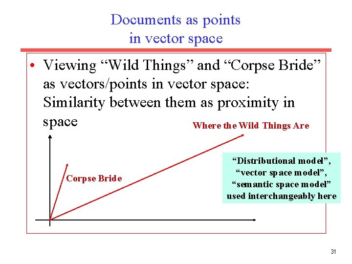
Documents as points in vector space • Viewing “Wild Things” and “Corpse Bride” as vectors/points in vector space: Similarity between them as proximity in space Where the Wild Things Are Corpse Bride “Distributional model”, “vector space model”, “semantic space model” used interchangeably here 31

What have we gained? • Representation of document in vector space can be computed completely automatically: Just counts words • Similarity in vector space is a good predictor for similarity in topic – Documents that contain similar words tend to be about similar things 32

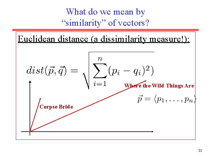
What do we mean by “similarity” of vectors? Euclidean distance (a dissimilarity measure!): Where the Wild Things Are Corpse Bride 33

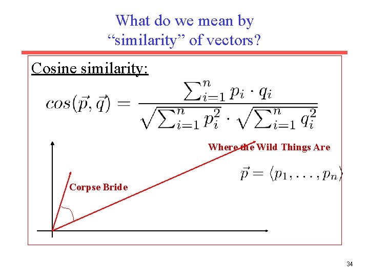
What do we mean by “similarity” of vectors? Cosine similarity: Where the Wild Things Are Corpse Bride 34

Now, to WSD One Idea • Create a vector based on counts in the training data for each sense of the target word – consider the words that appear within, say, 10 words of the target word. – So, rather than representing entire documents as vectors, we represent windows of, say, 10 words – E. g. , “finance” for the financial meanings of “bank” will have a higher count than it will for the “river bank” meaning of bank, since “finance” will appear more frequently near the financial meaning of “bank” • Represent each test instance as its own vector • Measure similarity between the test instance vector and each of the vectors created for each sense. Assign the sense for which similarity is greatest. 35

Summary: vector space models • Representing meaning through counts – Represent document/sentence/context through content words • Proximity in semantic space ~ similarity between words 36

Summary: vector space models • Uses: – – – Search Inducing ontologies Modeling human judgments of word similarity Improve supervised word sense disambiguation Word-sense discrimination: cluster words based on vectors; the clusters may not correspond to any particular sense inventory 37

Thesaurus-based word similarity • We could use anything in thesaurus – Meronymy – Glosses – Example sentences • In practice – By “thesaurus-based” we just mean • Using the is-a/subsumption/hypernym hierarchy • Can define similarity between words or between senses 38

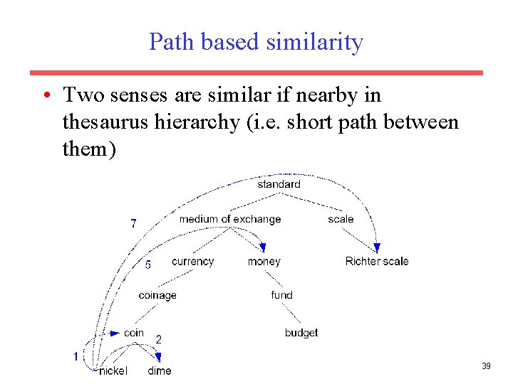
Path based similarity • Two senses are similar if nearby in thesaurus hierarchy (i. e. short path between them) 39

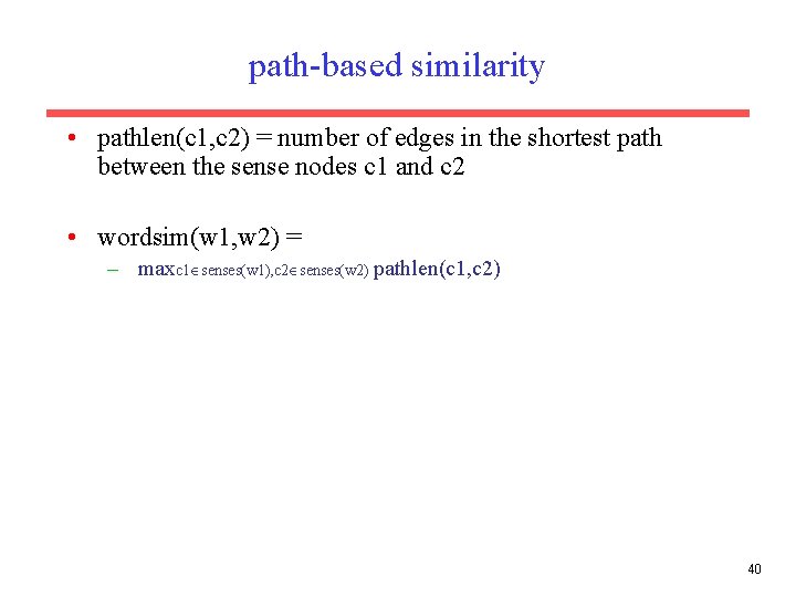
path-based similarity • pathlen(c 1, c 2) = number of edges in the shortest path between the sense nodes c 1 and c 2 • wordsim(w 1, w 2) = – maxc 1 senses(w 1), c 2 senses(w 2) pathlen(c 1, c 2) 40

Problem with basic path-based similarity • Assumes each link represents a uniform distance • But, some areas of Word. Net are more developed than others • Depended on the people who created it 41

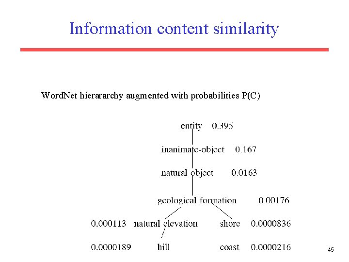
Information content similarity metrics • Let’s define P(C) as: – The probability that a randomly selected word in a corpus is an instance of concept c – A word is an instance of a concept if it appears below the concept in the Word. Net hierarchy – We saw this idea when we covered selectional preferences 42

In particular – P(root)=1 – The lower a node in the hierarchy, the lower its probability – An occurrence of the word dime would count towards the frequency of coin, currency, standard, etc. 43

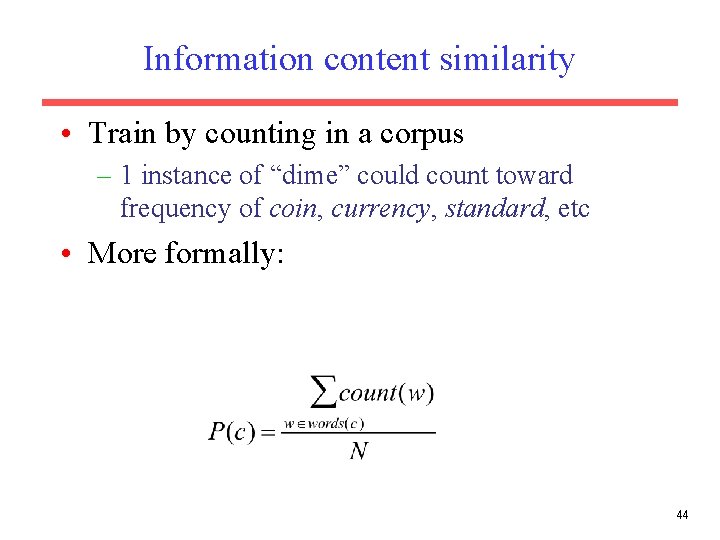
Information content similarity • Train by counting in a corpus – 1 instance of “dime” could count toward frequency of coin, currency, standard, etc • More formally: 44

Information content similarity Word. Net hierararchy augmented with probabilities P(C) 45

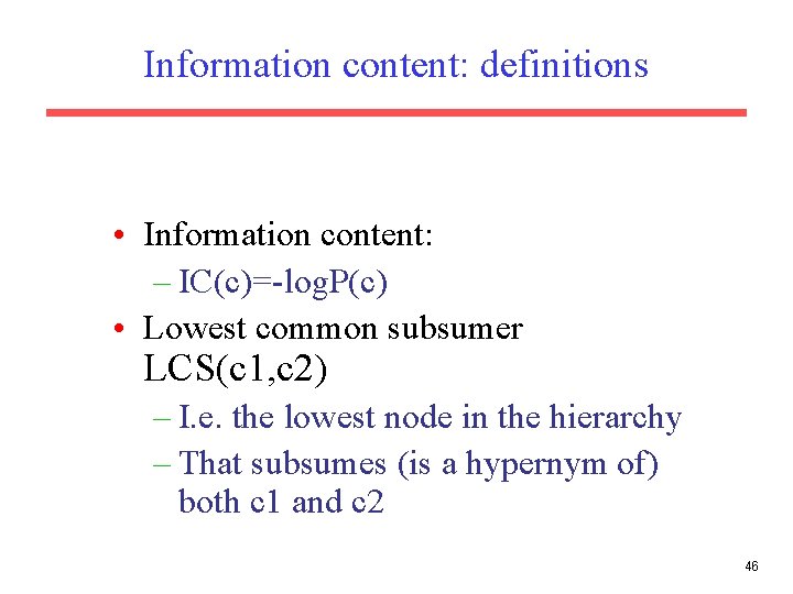
Information content: definitions • Information content: – IC(c)=-log. P(c) • Lowest common subsumer LCS(c 1, c 2) – I. e. the lowest node in the hierarchy – That subsumes (is a hypernym of) both c 1 and c 2 46

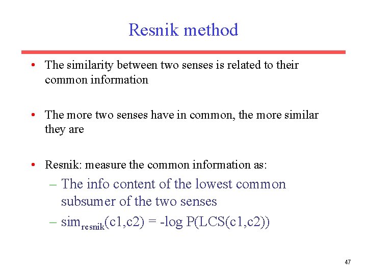
Resnik method • The similarity between two senses is related to their common information • The more two senses have in common, the more similar they are • Resnik: measure the common information as: – The info content of the lowest common subsumer of the two senses – simresnik(c 1, c 2) = -log P(LCS(c 1, c 2)) 47

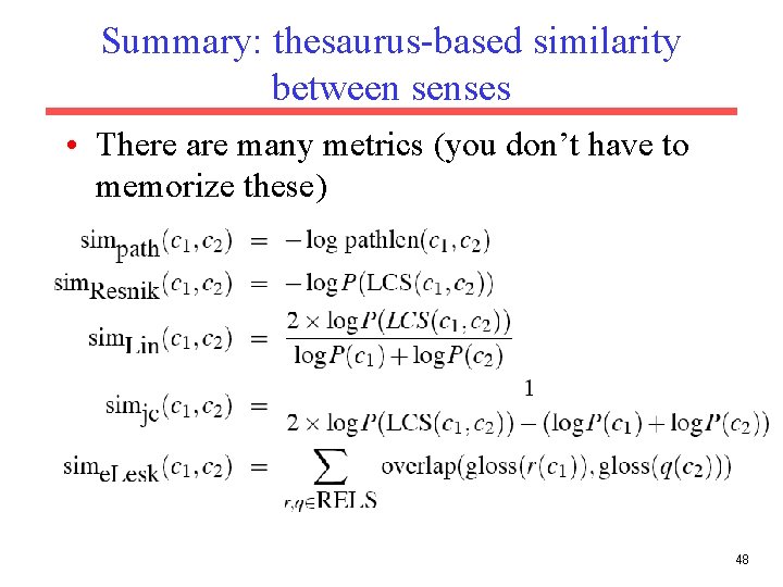
Summary: thesaurus-based similarity between senses • There are many metrics (you don’t have to memorize these) 48

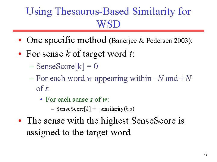
Using Thesaurus-Based Similarity for WSD • One specific method (Banerjee & Pedersen 2003): • For sense k of target word t: – Sense. Score[k] = 0 – For each word w appearing within –N and +N of t: • For each sense s of w: – Sense. Score[k] += similarity(k, s) • The sense with the highest Sense. Score is assigned to the target word 49

Evaluating Categorization • Evaluation must be done on test data that are independent of the training data (usually a disjoint set of instances). • Results can vary based on sampling error due to different training and test sets. • Average results over multiple training and test sets (splits of the overall data) for the best results. 50

N-Fold Cross-Validation • Ideally, test and training sets are independent on each trial. – But this would require too much labeled data. • Partition data into N equal-sized disjoint segments. • Run N trials, each time using a different segment of the data for testing, and training on the remaining N 1 segments. • This way, at least test-sets are independent. • Report average classification accuracy over the N trials. • Typically, N = 10. 51

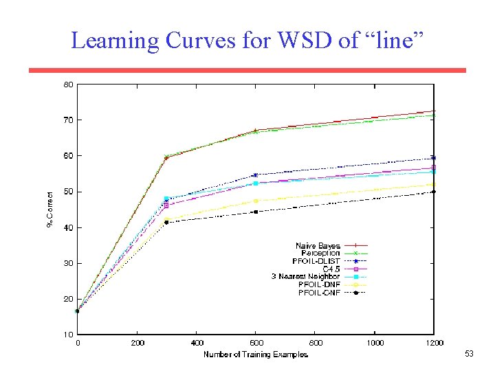
Learning Curves • In practice, labeled data is usually rare and expensive. • Would like to know how performance varies with the number of training instances. • Learning curves plot classification accuracy on independent test data (Y axis) versus number of training examples (X axis). 52

Learning Curves for WSD of “line” 53

Sense. Eval • Standardized international “competition” on WSD. • Organized by the Association for Computational Linguistics (ACL) Special Interest Group on the Lexicon (SIGLEX). – – Senseval 1: 1998 Senseval 2: 2001 Senseval 3: 2004 Senseval 4: 2007 54

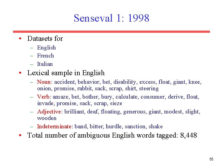
Senseval 1: 1998 • Datasets for – English – French – Italian • Lexical sample in English – Noun: accident, behavior, bet, disability, excess, float, giant, knee, onion, promise, rabbit, sack, scrap, shirt, steering – Verb: amaze, bet, bother, bury, calculate, consumer, derive, float, invade, promise, sack, scrap, sieze – Adjective: brilliant, deaf, floating, generous, giant, modest, slight, wooden – Indeterminate: band, bitter, hurdle, sanction, shake • Total number of ambiguous English words tagged: 8, 448 55

Senseval 1 English Sense Inventory • Senses from the HECTOR lexicography project. • Multiple levels of granularity – Coarse grained (avg. 7. 2 senses per word) – Fine grained (avg. 10. 4 senses per word) 56

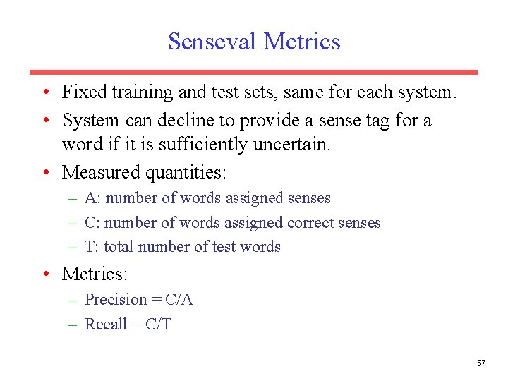
Senseval Metrics • Fixed training and test sets, same for each system. • System can decline to provide a sense tag for a word if it is sufficiently uncertain. • Measured quantities: – A: number of words assigned senses – C: number of words assigned correct senses – T: total number of test words • Metrics: – Precision = C/A – Recall = C/T 57

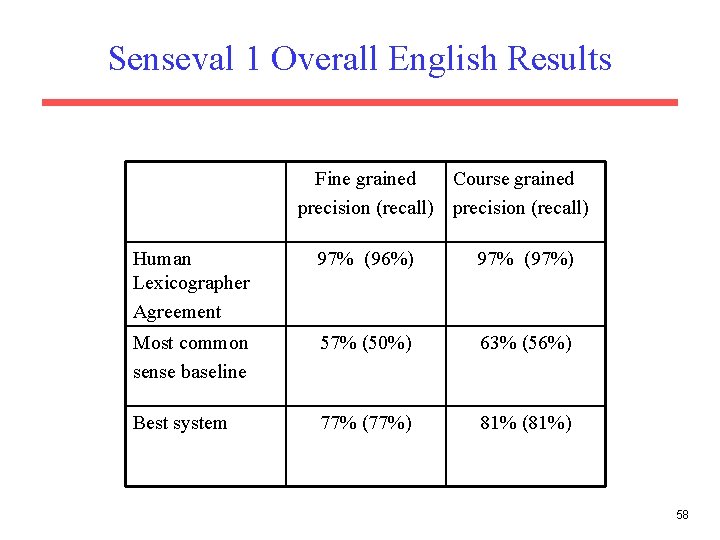
Senseval 1 Overall English Results Fine grained Course grained precision (recall) Human Lexicographer Agreement 97% (96%) 97% (97%) Most common sense baseline 57% (50%) 63% (56%) Best system 77% (77%) 81% (81%) 58

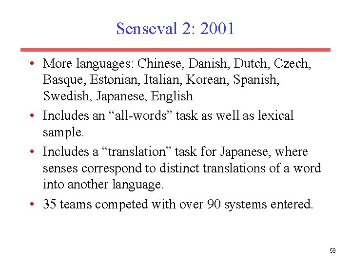
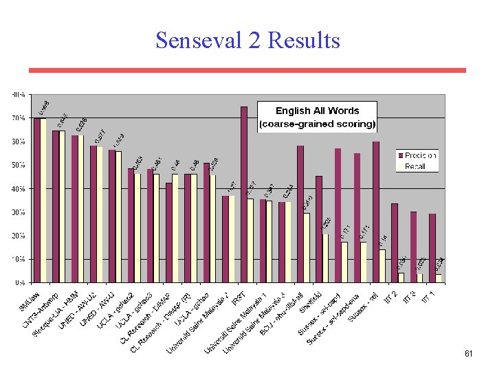
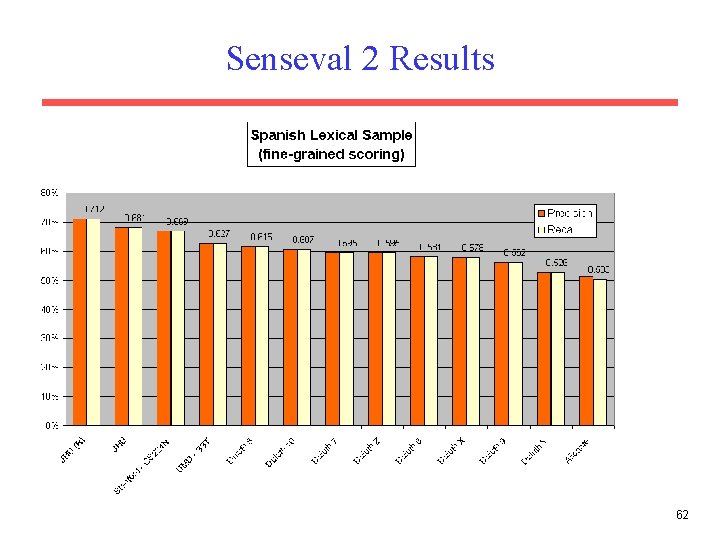
Senseval 2: 2001 • More languages: Chinese, Danish, Dutch, Czech, Basque, Estonian, Italian, Korean, Spanish, Swedish, Japanese, English • Includes an “all-words” task as well as lexical sample. • Includes a “translation” task for Japanese, where senses correspond to distinct translations of a word into another language. • 35 teams competed with over 90 systems entered. 59

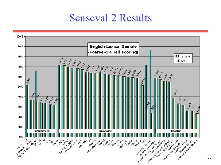
Senseval 2 Results 60

Senseval 2 Results 61

Senseval 2 Results 62

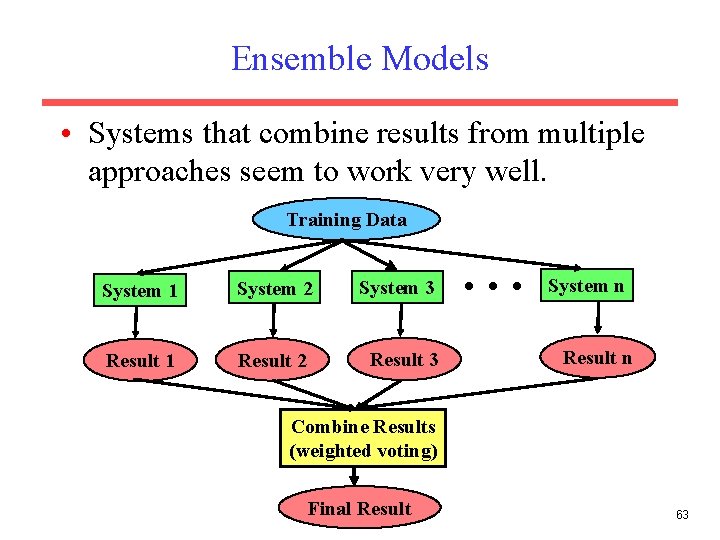
Ensemble Models • Systems that combine results from multiple approaches seem to work very well. Training Data System 1 System 2 System 3 Result 1 Result 2 Result 3 . . . System n Result n Combine Results (weighted voting) Final Result 63

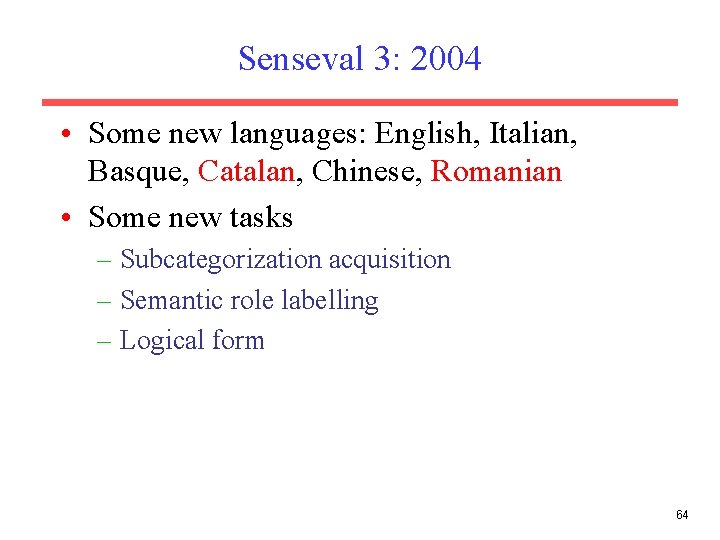
Senseval 3: 2004 • Some new languages: English, Italian, Basque, Catalan, Chinese, Romanian • Some new tasks – Subcategorization acquisition – Semantic role labelling – Logical form 64

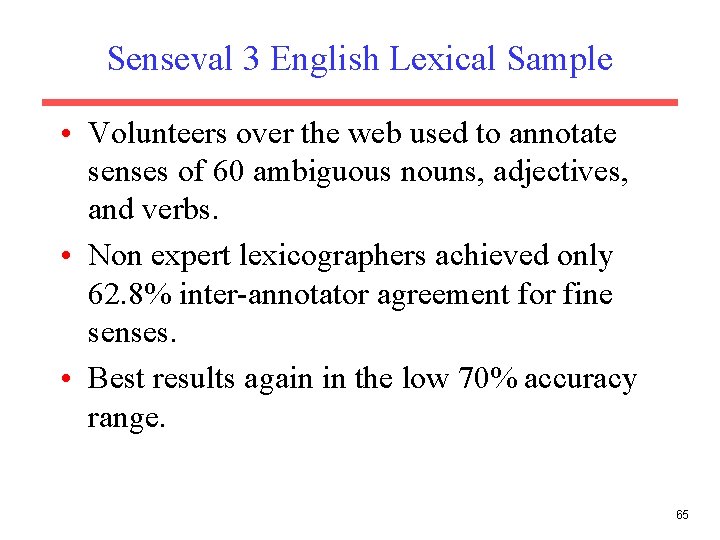
Senseval 3 English Lexical Sample • Volunteers over the web used to annotate senses of 60 ambiguous nouns, adjectives, and verbs. • Non expert lexicographers achieved only 62. 8% inter-annotator agreement for fine senses. • Best results again in the low 70% accuracy range. 65

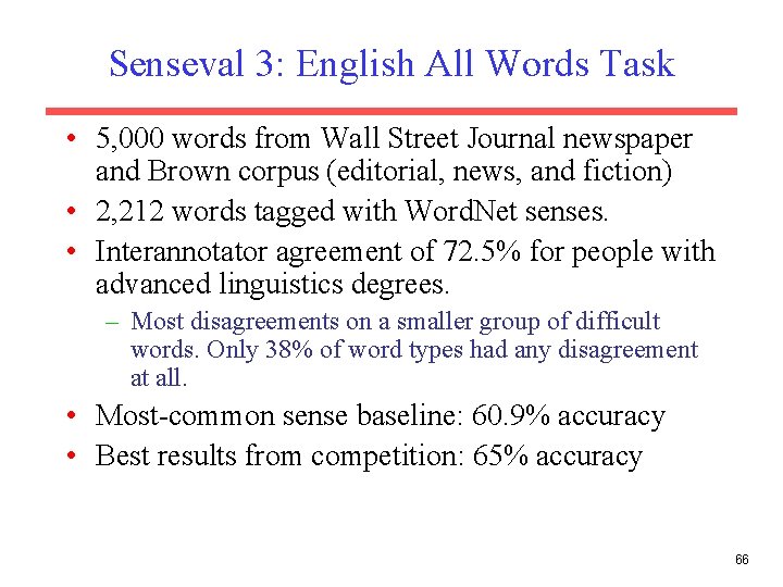
Senseval 3: English All Words Task • 5, 000 words from Wall Street Journal newspaper and Brown corpus (editorial, news, and fiction) • 2, 212 words tagged with Word. Net senses. • Interannotator agreement of 72. 5% for people with advanced linguistics degrees. – Most disagreements on a smaller group of difficult words. Only 38% of word types had any disagreement at all. • Most-common sense baseline: 60. 9% accuracy • Best results from competition: 65% accuracy 66

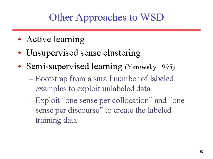
Other Approaches to WSD • Active learning • Unsupervised sense clustering • Semi-supervised learning (Yarowsky 1995) – Bootstrap from a small number of labeled examples to exploit unlabeled data – Exploit “one sense per collocation” and “one sense per discourse” to create the labeled training data 67

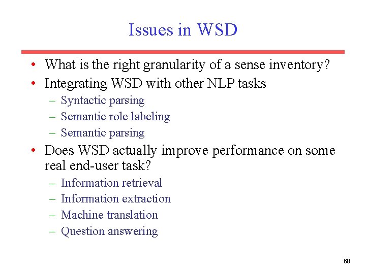
Issues in WSD • What is the right granularity of a sense inventory? • Integrating WSD with other NLP tasks – Syntactic parsing – Semantic role labeling – Semantic parsing • Does WSD actually improve performance on some real end-user task? – – Information retrieval Information extraction Machine translation Question answering 68