Chapter 2 Valuing the Environment Concepts Environmental Economics
- Slides: 22

Chapter 2 Valuing the Environment: Concepts Environmental Economics and Policy Sixth Edition By Tom Tietenberg and Lynne Lewis Copyright © 2010 Pearson Addison-Wesley. All rights reserved.

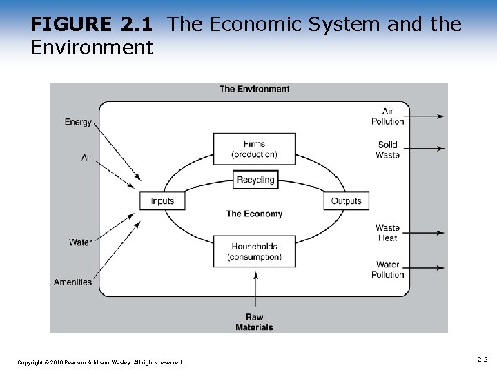
FIGURE 2. 1 The Economic System and the Environment 1 -2 Copyright © 2010 Pearson Addison-Wesley. All rights reserved. 2 -2

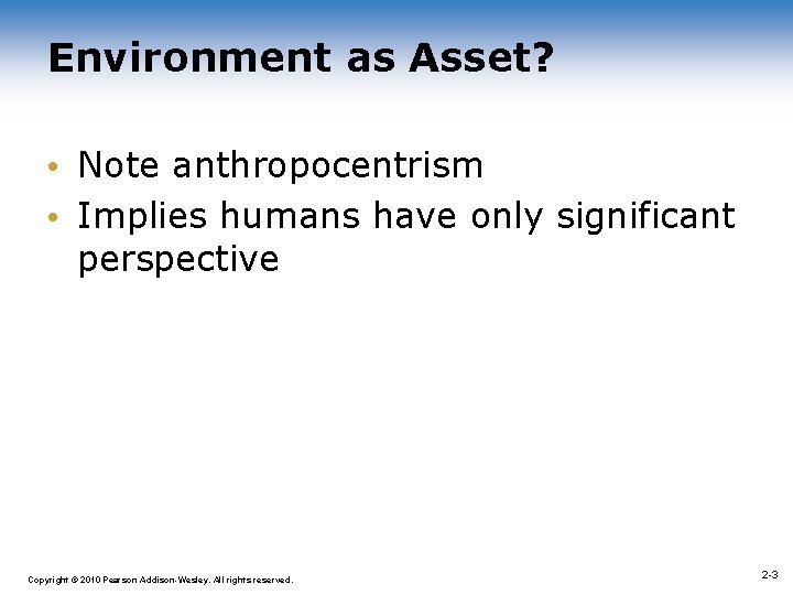
Environment as Asset? • Note anthropocentrism • Implies humans have only significant perspective 1 -3 Copyright © 2010 Pearson Addison-Wesley. All rights reserved. 2 -3

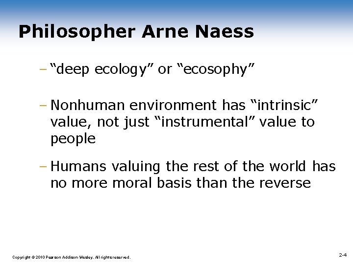
Philosopher Arne Naess – “deep ecology” or “ecosophy” – Nonhuman environment has “intrinsic” value, not just “instrumental” value to people – Humans valuing the rest of the world has no more moral basis than the reverse 1 -4 Copyright © 2010 Pearson Addison-Wesley. All rights reserved. 2 -4

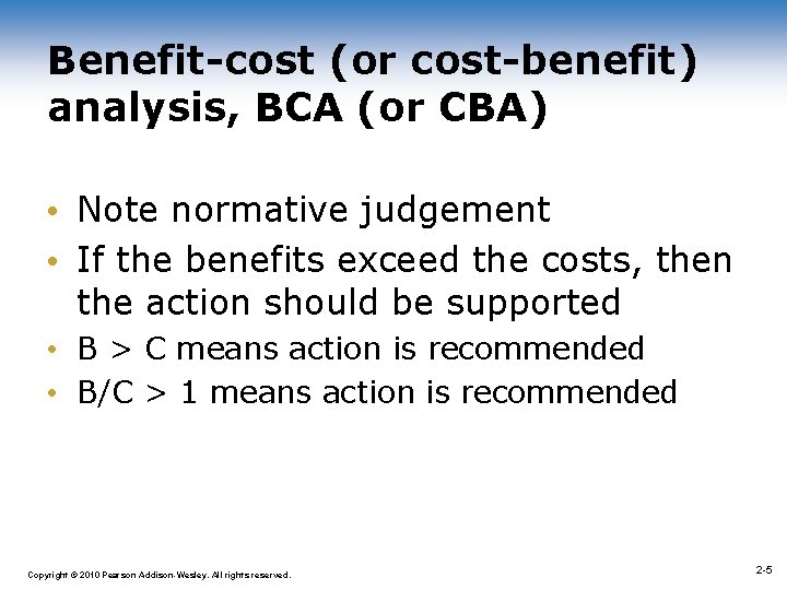
Benefit-cost (or cost-benefit) analysis, BCA (or CBA) • Note normative judgement • If the benefits exceed the costs, then the action should be supported • B > C means action is recommended • B/C > 1 means action is recommended 1 -5 Copyright © 2010 Pearson Addison-Wesley. All rights reserved. 2 -5

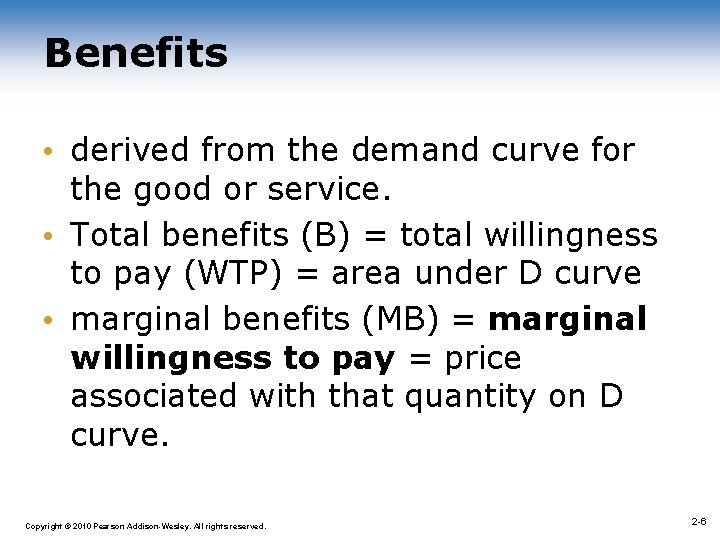
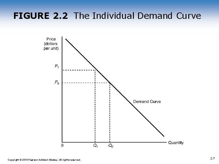
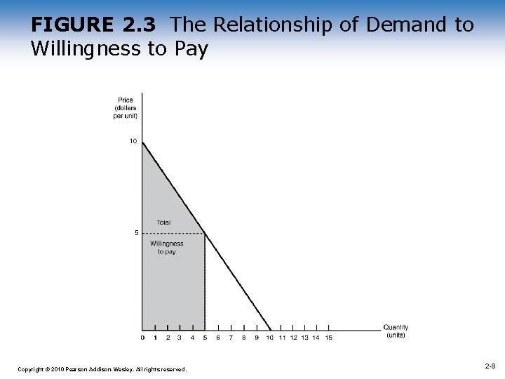
Benefits • derived from the demand curve for the good or service. • Total benefits (B) = total willingness to pay (WTP) = area under D curve • marginal benefits (MB) = marginal willingness to pay = price associated with that quantity on D curve. 1 -6 Copyright © 2010 Pearson Addison-Wesley. All rights reserved. 2 -6

FIGURE 2. 2 The Individual Demand Curve 1 -7 Copyright © 2010 Pearson Addison-Wesley. All rights reserved. 2 -7

FIGURE 2. 3 The Relationship of Demand to Willingness to Pay 1 -8 Copyright © 2010 Pearson Addison-Wesley. All rights reserved. 2 -8

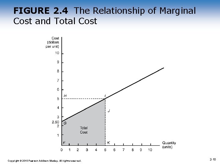
Costs • derived from the marginal cost (supply) curve for the good or service • Total costs = area under MC (Marginal Cost) curve • Marginal opportunity cost is the cost of producing the last unit = point on MC curve associated with that Q. 1 -9 Copyright © 2010 Pearson Addison-Wesley. All rights reserved. 2 -9

FIGURE 2. 4 The Relationship of Marginal Cost and Total Cost 1 -10 Copyright © 2010 Pearson Addison-Wesley. All rights reserved. 2 -10

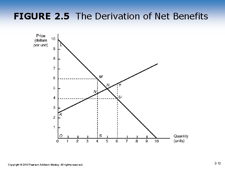
Net benefit • the excess of benefits over costs • the area under the demand curve that lies above the supply curve • consumer plus producer surplus 1 -11 Copyright © 2010 Pearson Addison-Wesley. All rights reserved. 2 -11

FIGURE 2. 5 The Derivation of Net Benefits 1 -12 Copyright © 2010 Pearson Addison-Wesley. All rights reserved. 2 -12

Issues with a time dimension • Present value is a method for evaluating benefits and costs occurring at different points in time • Allows us to compare dollars today to dollars in some future period by translating everything back to its current worth. Then apply benefitcost analysis. 1 -13 Copyright © 2010 Pearson Addison-Wesley. All rights reserved. 2 -13

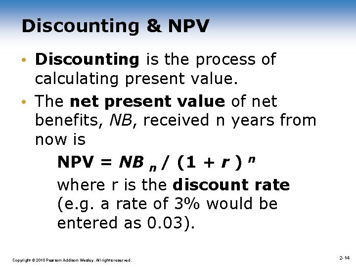
Discounting & NPV • Discounting is the process of calculating present value. • The net present value of net benefits, NB, received n years from now is NPV = NB n / (1 + r ) n where r is the discount rate (e. g. a rate of 3% would be entered as 0. 03). 1 -14 Copyright © 2010 Pearson Addison-Wesley. All rights reserved. 2 -14

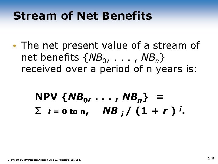
Stream of Net Benefits • The net present value of a stream of net benefits {NB 0, . . . , NBn} received over a period of n years is: NPV {NB 0, . . . , NBn} = Σ i = 0 to n, NB i / (1 + r ) i. 1 -15 Copyright © 2010 Pearson Addison-Wesley. All rights reserved. 2 -15

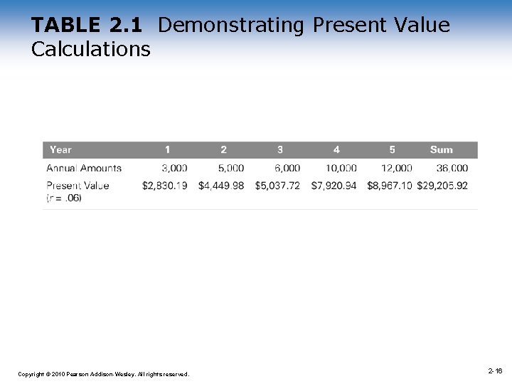
TABLE 2. 1 Demonstrating Present Value Calculations 1 -16 Copyright © 2010 Pearson Addison-Wesley. All rights reserved. 2 -16

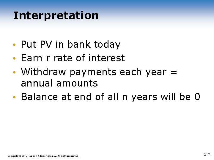
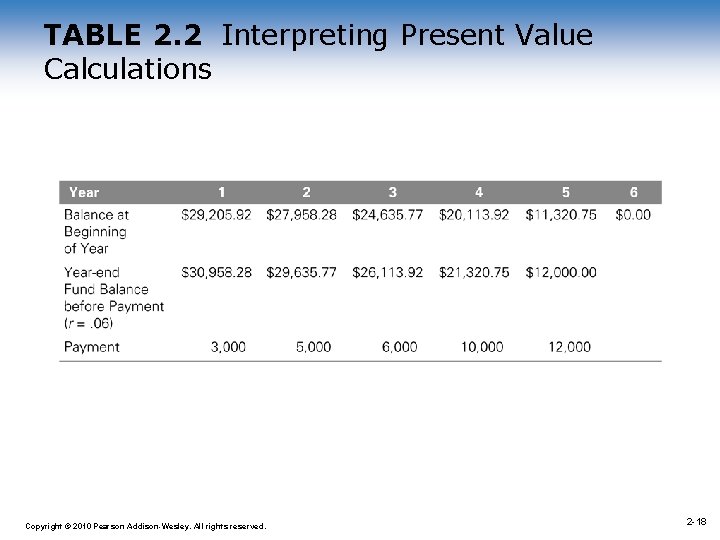
Interpretation • Put PV in bank today • Earn r rate of interest • Withdraw payments each year = annual amounts • Balance at end of all n years will be 0 1 -17 Copyright © 2010 Pearson Addison-Wesley. All rights reserved. 2 -17

TABLE 2. 2 Interpreting Present Value Calculations 1 -18 Copyright © 2010 Pearson Addison-Wesley. All rights reserved. 2 -18

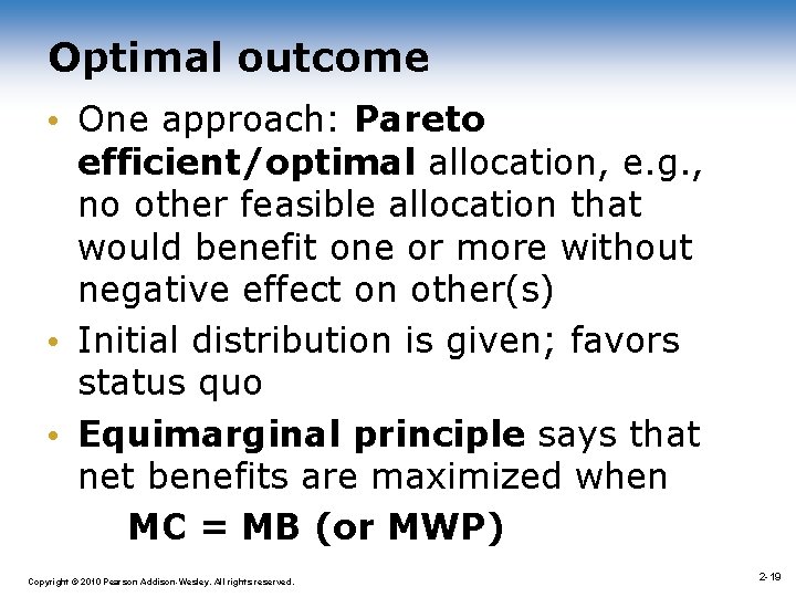
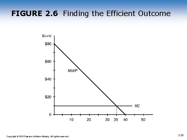
Optimal outcome • One approach: Pareto efficient/optimal allocation, e. g. , no other feasible allocation that would benefit one or more without negative effect on other(s) • Initial distribution is given; favors status quo • Equimarginal principle says that net benefits are maximized when MC = MB (or MWP) Copyright © 2010 Pearson Addison-Wesley. All rights reserved. 1 -19 2 -19

FIGURE 2. 6 Finding the Efficient Outcome 1 -20 Copyright © 2010 Pearson Addison-Wesley. All rights reserved. 2 -20

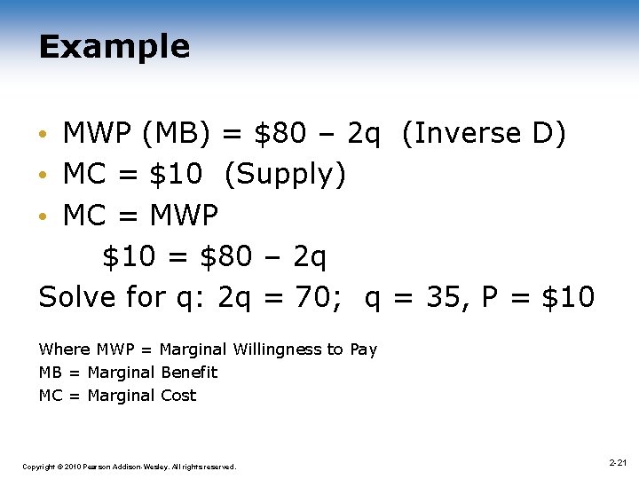
Example • MWP (MB) = $80 – 2 q (Inverse D) • MC = $10 (Supply) • MC = MWP $10 = $80 – 2 q Solve for q: 2 q = 70; q = 35, P = $10 Where MWP = Marginal Willingness to Pay MB = Marginal Benefit MC = Marginal Cost 1 -21 Copyright © 2010 Pearson Addison-Wesley. All rights reserved. 2 -21

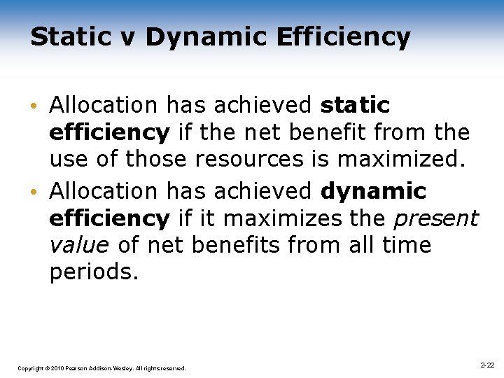
Static v Dynamic Efficiency • Allocation has achieved static efficiency if the net benefit from the use of those resources is maximized. • Allocation has achieved dynamic efficiency if it maximizes the present value of net benefits from all time periods. 1 -22 Copyright © 2010 Pearson Addison-Wesley. All rights reserved. 2 -22