Chapter 2 Utility and Choice Theory of Choice

Chapter 2 Utility and Choice

Theory of Choice l 2 The interaction of preferences and constraints that causes people to make the choices they do

Utility l l l 3 The pleasure, satisfaction, or need fulfillment that people get from their economic activity. To identify all of the factors that affect utility would be virtually impossible Much economic analysis is based on the ceteris paribus assumption.

Ceteris Paribus Assumption l l 4 In economic analysis, holding all other factors constant so that only the factor being studied is allowed to change Other factors are held constant so that we may choose a simple setting that isolates the economic factors that affect behavior

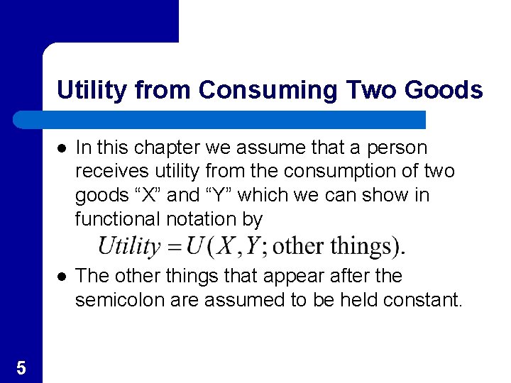
Utility from Consuming Two Goods 5 l In this chapter we assume that a person receives utility from the consumption of two goods “X” and “Y” which we can show in functional notation by l The other things that appear after the semicolon are assumed to be held constant.

Measuring Utility l Two problems make it difficult to measure utility directly. – – l 6 Because the real-world is constantly in flux, the ceteris paribus assumption is difficult to impose. There is no unit of utility measurement. However, it is possible to do a fairly complete job of studying choices without having to measure utility.

Assumptions about Utility l Basic Properties of Preferences – – 7 Preferences are complete : The assumption that an individual is able to state which of any two options is preferred. Preferences are transitive: The property that if A is preferred to B, and B is preferred to C, then A must be preferred to C.

Application 2. 1: Can Money Buy Health and Happiness? l l l 8 The relationship between health and income has been intensely studied Virtually all of these studies conclude that people who have higher incomes have better health People with higher incomes tend to report that they are happier than are those with lower incomes.

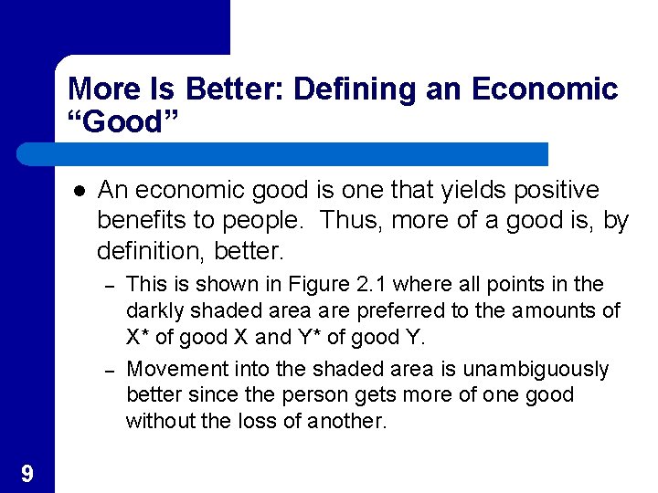
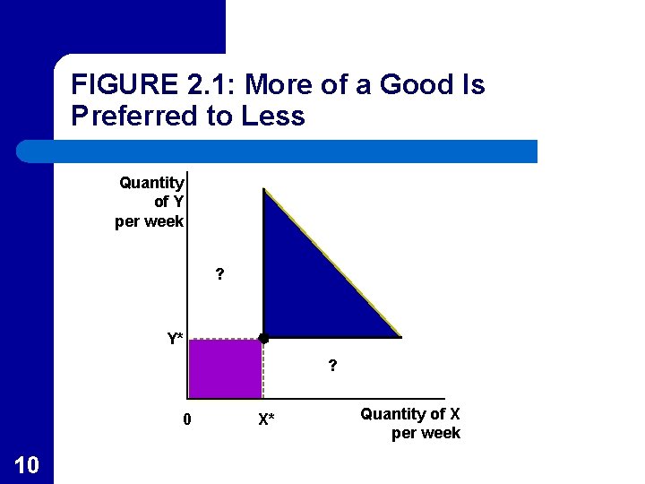
More Is Better: Defining an Economic “Good” l An economic good is one that yields positive benefits to people. Thus, more of a good is, by definition, better. – – 9 This is shown in Figure 2. 1 where all points in the darkly shaded area are preferred to the amounts of X* of good X and Y* of good Y. Movement into the shaded area is unambiguously better since the person gets more of one good without the loss of another.

FIGURE 2. 1: More of a Good Is Preferred to Less Quantity of Y per week ? Y* ? 0 10 X* Quantity of X per week

Voluntary Trades and Indifference Curves l l 11 The areas marked with question marks in Figure 2. 1 are difficult to compare to X*, Y* since they involve more of one good but less of another. Trading one good (such as money) for another good (such as a candy bar) is the essence of demand.

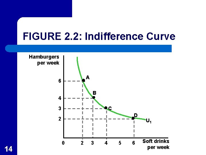
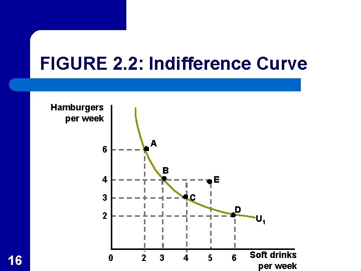
Indifference Curves l l 12 A curve that shows all the combinations of goods or services that provide the same level of utility. In Figure 2. 2, the horizontal axis measures the quantity of soft drinks consumed by the individual per week while the vertical axis measures the quantity of hamburgers consumed per week.

Indifference Curves l The curve U 1 in Figure 2. 2 includes all combinations of hamburgers and soft drinks that yield the same level of utility. – – 13 Point A, with 6 hamburgers and 2 soft drinks, has the same utility as point B, 4 burgers and 3 drinks. Since all points on the curve yield the same utility, the person has no reason to prefer one point over another.

FIGURE 2. 2: Indifference Curve Hamburgers per week A 6 B 4 3 C D 2 14 0 2 3 4 5 6 U 1 Soft drinks per week

Points Above an Indifference Curve l In Figure 2. 2, points such as E are above (to the northeast) of U 1. – – – 15 Since E has more of both goods than point C, E is preferred to C (more is better). Because of transitivity, E is preferred to any point on U 1. Points above an indifference curve are preferred to points on the curve.

FIGURE 2. 2: Indifference Curve Hamburgers per week A 6 B 4 E 3 C D 2 16 0 2 3 4 5 6 U 1 Soft drinks per week

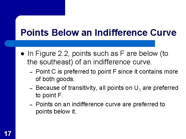
Points Below an Indifference Curve l In Figure 2. 2, points such as F are below (to the southeast) of an indifference curve. – – – 17 Point C is preferred to point F since it contains more of both goods. Because of transitivity, all points on U 1 are preferred to point F. Points on an indifference curve are preferred to points below it.

FIGURE 2. 2: Indifference Curve Hamburgers per week A 6 B 4 E 3 C 18 D F 2 0 2 3 4 5 6 U 1 Soft drinks per week

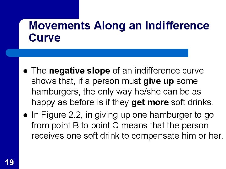
Movements Along an Indifference Curve l l 19 The negative slope of an indifference curve shows that, if a person must give up some hamburgers, the only way he/she can be as happy as before is if they get more soft drinks. In Figure 2. 2, in giving up one hamburger to go from point B to point C means that the person receives one soft drink to compensate him or her.

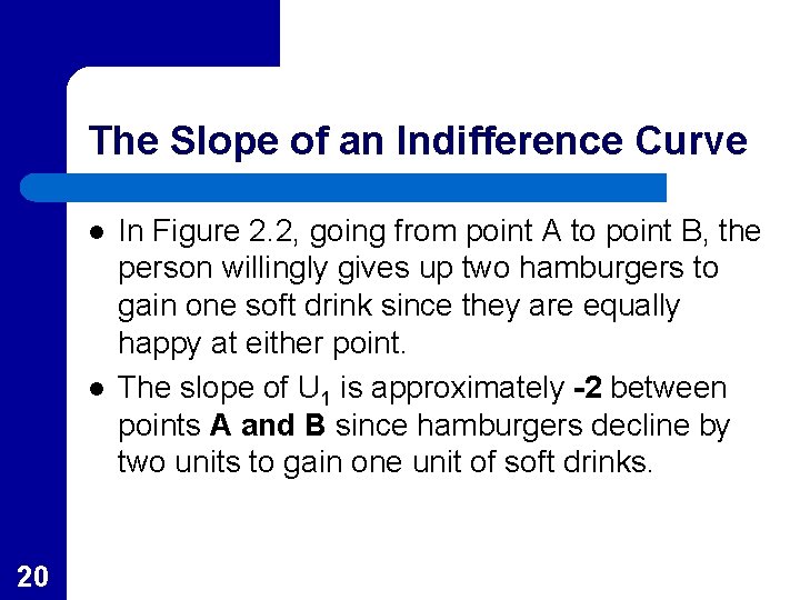
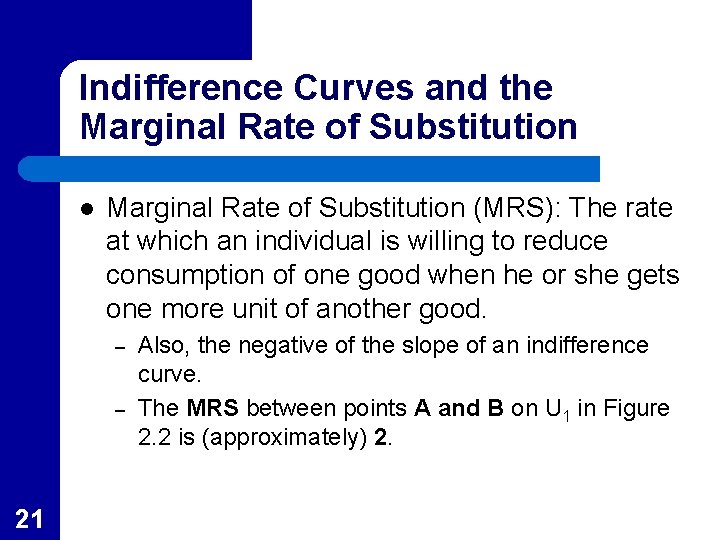
The Slope of an Indifference Curve l l 20 In Figure 2. 2, going from point A to point B, the person willingly gives up two hamburgers to gain one soft drink since they are equally happy at either point. The slope of U 1 is approximately -2 between points A and B since hamburgers decline by two units to gain one unit of soft drinks.

Indifference Curves and the Marginal Rate of Substitution l Marginal Rate of Substitution (MRS): The rate at which an individual is willing to reduce consumption of one good when he or she gets one more unit of another good. – – 21 Also, the negative of the slope of an indifference curve. The MRS between points A and B on U 1 in Figure 2. 2 is (approximately) 2.

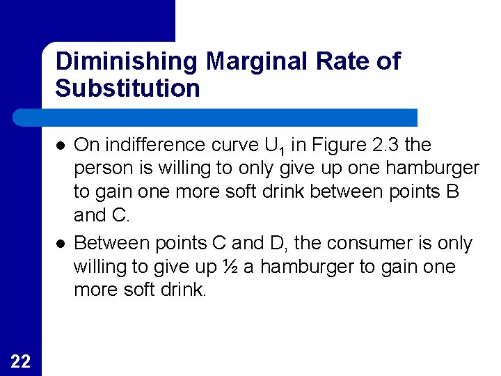
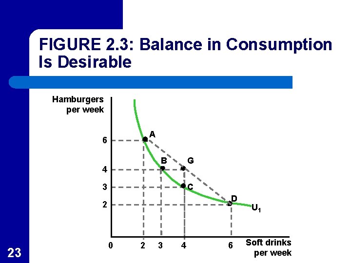
Diminishing Marginal Rate of Substitution l l 22 On indifference curve U 1 in Figure 2. 3 the person is willing to only give up one hamburger to gain one more soft drink between points B and C. Between points C and D, the consumer is only willing to give up ½ a hamburger to gain one more soft drink.

FIGURE 2. 3: Balance in Consumption Is Desirable Hamburgers per week A 6 B 4 G 3 C D 2 23 0 2 3 4 6 U 1 Soft drinks per week

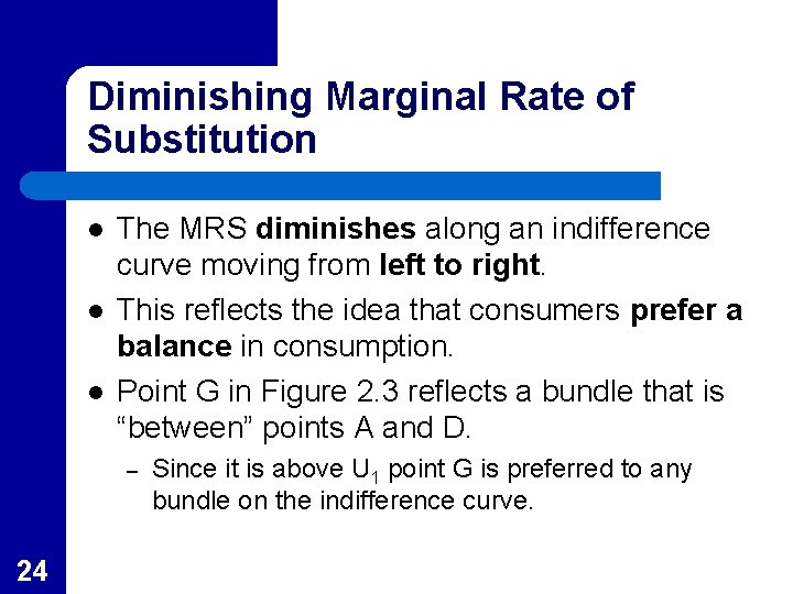
Diminishing Marginal Rate of Substitution l l l The MRS diminishes along an indifference curve moving from left to right. This reflects the idea that consumers prefer a balance in consumption. Point G in Figure 2. 3 reflects a bundle that is “between” points A and D. – 24 Since it is above U 1 point G is preferred to any bundle on the indifference curve.

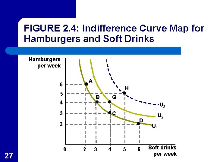
Indifference Curve Maps l l Since every combination of hamburgers and soft drinks must yield some level of utility, every point must have one (and only one) indifference curve passing through it. An indifference curve map shows the utility an individual obtains from all possible consumption options. – 25 Figure 2. 4 shows three of the infinite number of indifference curves in the map.

Labeling Indifference Curves l l 26 Since utility can not be measured, the labeling of indifference curves has no meaning except to indicate that utility increases from U 1 to U 2 and then to U 3 in Figure 2. 4. In any indifference curve map, all we can assume is that utility increases as we move to higher indifference curves.

FIGURE 2. 4: Indifference Curve Map for Hamburgers and Soft Drinks Hamburgers per week A 6 H 5 B 4 G U 3 3 C D 2 27 0 2 3 4 5 6 U 2 U 1 Soft drinks per week

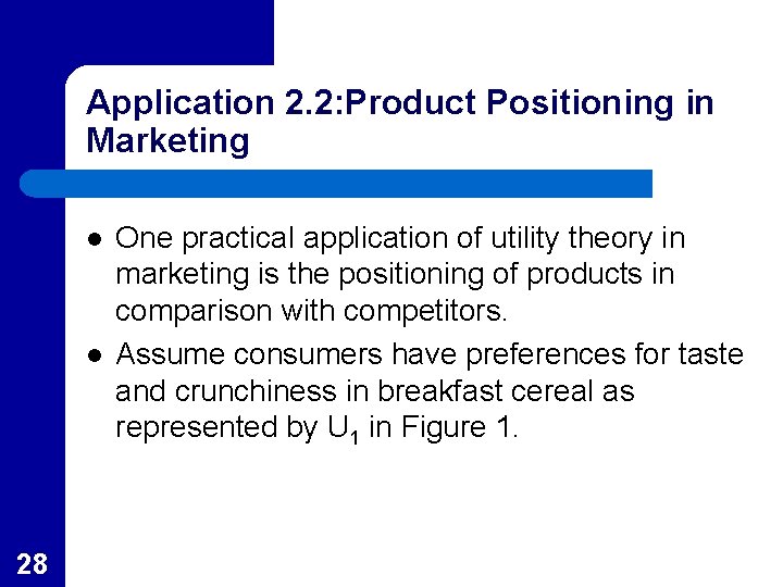
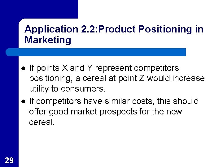
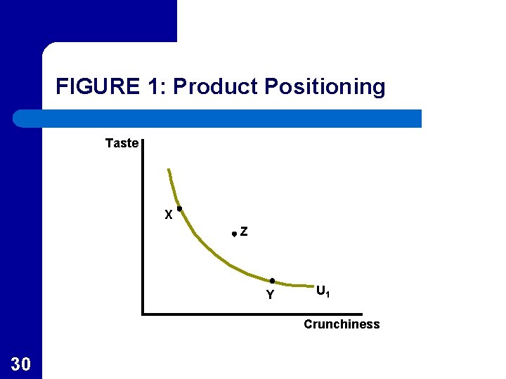
Application 2. 2: Product Positioning in Marketing l l 28 One practical application of utility theory in marketing is the positioning of products in comparison with competitors. Assume consumers have preferences for taste and crunchiness in breakfast cereal as represented by U 1 in Figure 1.

Application 2. 2: Product Positioning in Marketing l l 29 If points X and Y represent competitors, positioning, a cereal at point Z would increase utility to consumers. If competitors have similar costs, this should offer good market prospects for the new cereal.

FIGURE 1: Product Positioning Taste X Z Y U 1 Crunchiness 30

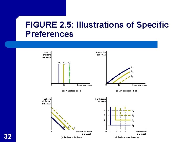
Illustrating Particular Preferences l l 31 In Figure 2. 5(a) the good on the vertical axis (smoke grinders) is useless so that the consumers only gains utility from more of the good on the horizontal axis (food). In Figure 2. 5(b) the good on the vertical axis is an economic bad (houseflies) so the consumer only gets more utility from consuming less of the bad.

FIGURE 2. 5: Illustrations of Specific Preferences Smoke grinders per week Houseflies per week U 1 U 2 U 3 0 10 Food per week 0 10 (a) A useless good Gallons of Exxon per week 32 (b) An economic bad Right shoes per week U 1 0 Food per week U 2 4 U 4 3 U 3 2 U 2 1 U 3 Gallons of Mobil per week (c) Perfect substitute 0 1 2 3 4 Left shoes per week (d) Perfect complements

Particular Preferences l In Figure 2. 5(c) the two goods are perfect substitutes in that the consumer views them as essentially the same. – l 33 In this example the MRS = 1. In Figure 2. 5(d) the two goods are perfect complements in that they must be used together (like left and right shoes) to gain utility.

Utility Maximization: An Initial Survey l l 34 Economists assume that when a person is faced with a choice among several possible options, he or she will choose the one that yields the highest utility- utility maximization. Economists assume that people know their own minds and make choices consistent with their preferences.

Choices are Constrained l l 35 People are constrained in their choices by the size of their incomes. Of the choices the individual can afford, the person will choose the one that yields the most utility.

A Simple Case l When choosing to allocate income between two goods (e. g. hamburgers and soft drinks) the consumer will: – – 36 spend his or her entire income on the two goods, and choose a combination of goods for which the marginal rate of substitution between the two goods is equal to the ratio of their prices.

A Simple Case l l 37 Since both goods (and only these goods) provide more utility with increased consumption the consumer will spend his or her entire income on the goods. The only other alternative is to throw the income away which does not increase utility.

Equality of MRS with the Ratio or Prices l l l 38 Suppose the individual is currently consuming where MRS = 1. Assume the price of hamburgers is $1 and the price of soft drinks is $. 50. This yields a price ratio (PS/PH) of ($. 50/$1) = ½.

Equality of MRS with the Ratio or Prices l The person could give up one hamburger (freeing $1) and purchase one soft drink using $. 50. – l 39 Since his or her MRS =1, the person would be just as happy as before but would now have an additional $. 50 to spend which would enable him or her to increase utility. The only way utility can not be increased further is when MRS = price ratio!!.

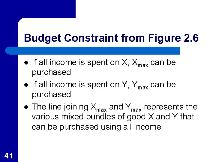
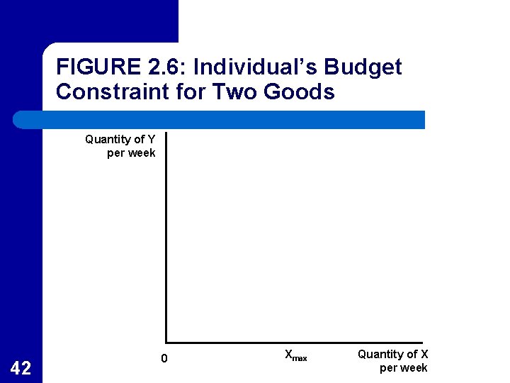
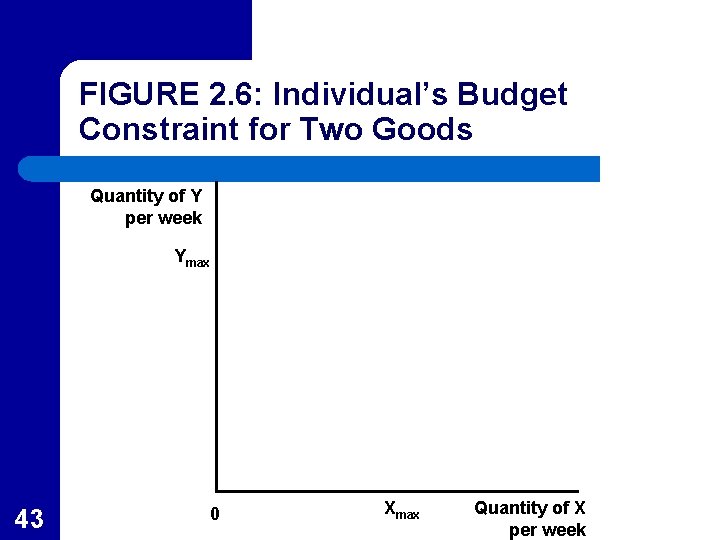
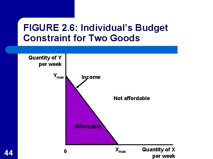
Graphic Analysis of Utility Maximization l l 40 An individual’s budget constraint is the limit that income places on the combinations of goods and services that a person can buy. In Figure 2. 6 the individual has a fixed amount of income that can be spend on two goods, X and Y.

Budget Constraint from Figure 2. 6 l l l 41 If all income is spent on X, Xmax can be purchased. If all income is spent on Y, Ymax can be purchased. The line joining Xmax and Ymax represents the various mixed bundles of good X and Y that can be purchased using all income.

FIGURE 2. 6: Individual’s Budget Constraint for Two Goods Quantity of Y per week 42 0 Xmax Quantity of X per week

FIGURE 2. 6: Individual’s Budget Constraint for Two Goods Quantity of Y per week Ymax 43 0 Xmax Quantity of X per week

FIGURE 2. 6: Individual’s Budget Constraint for Two Goods Quantity of Y per week Ymax Income Not affordable Affordable 44 0 Xmax Quantity of X per week

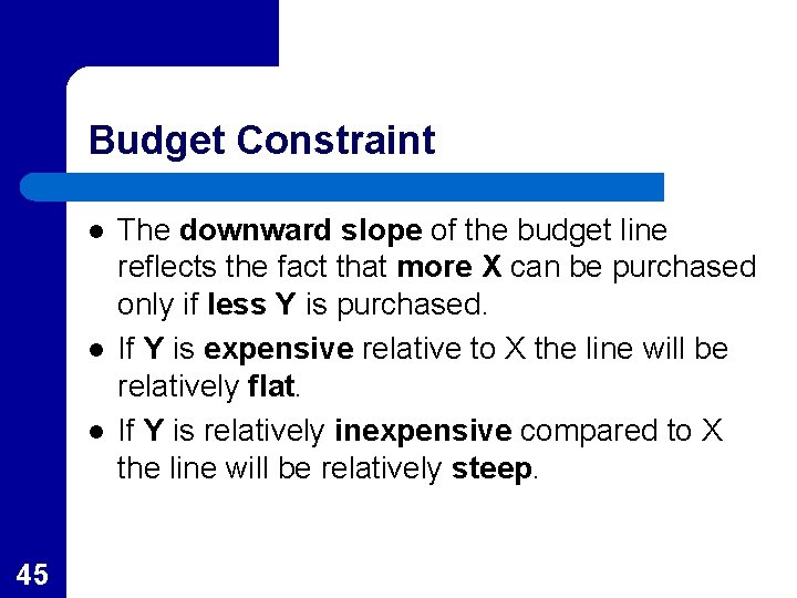
Budget Constraint l l l 45 The downward slope of the budget line reflects the fact that more X can be purchased only if less Y is purchased. If Y is expensive relative to X the line will be relatively flat. If Y is relatively inexpensive compared to X the line will be relatively steep.

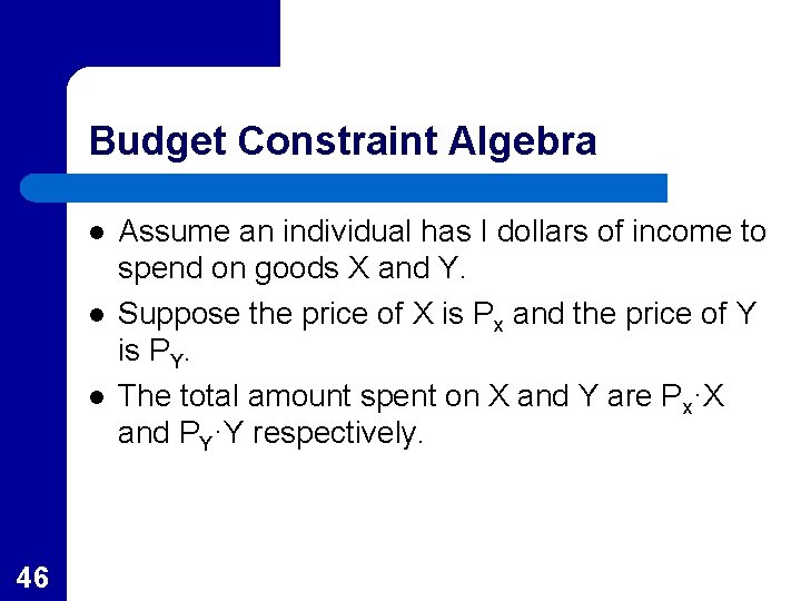
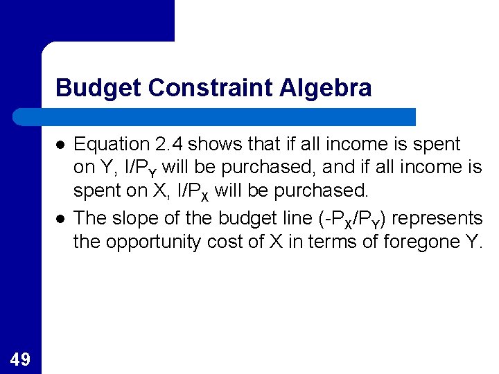
Budget Constraint Algebra l l l 46 Assume an individual has I dollars of income to spend on goods X and Y. Suppose the price of X is Px and the price of Y is PY. The total amount spent on X and Y are Px·X and PY·Y respectively.

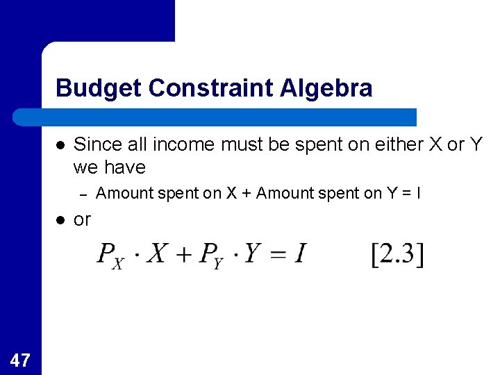
Budget Constraint Algebra l Since all income must be spent on either X or Y we have – l 47 or Amount spent on X + Amount spent on Y = I

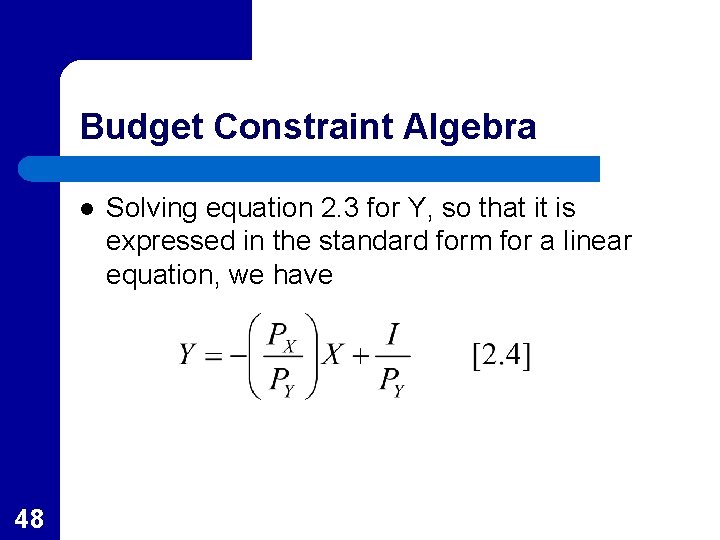
Budget Constraint Algebra l 48 Solving equation 2. 3 for Y, so that it is expressed in the standard form for a linear equation, we have

Budget Constraint Algebra l l 49 Equation 2. 4 shows that if all income is spent on Y, I/PY will be purchased, and if all income is spent on X, I/PX will be purchased. The slope of the budget line (-PX/PY) represents the opportunity cost of X in terms of foregone Y.

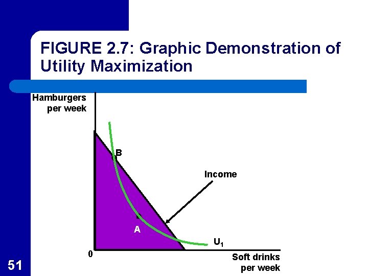
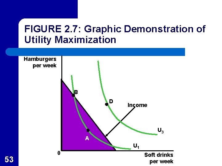
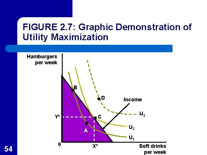
Utility Maximization l l l 50 An individual can afford all bundles of X and Y that fall within the budget constraint represented by the shaded area in Figure 2. 6. Point A is affordable but not all of the consumer’s income would be spent. Point B is affordable but is not on the highest indifference curve that can be reached by the consumer.

FIGURE 2. 7: Graphic Demonstration of Utility Maximization Hamburgers per week B Income A U 1 51 0 Soft drinks per week

Utility Maximization l l 52 Point D is on a higher indifference curve than C, but is not affordable given the budget constraint. Point C, where the consumer chooses X*, Y* is the point that is affordable that lies on the highest indifference curve, so it represents utility maximization.

FIGURE 2. 7: Graphic Demonstration of Utility Maximization Hamburgers per week B D Income U 3 A U 1 53 0 Soft drinks per week

FIGURE 2. 7: Graphic Demonstration of Utility Maximization Hamburgers per week B D Y* Income U 3 C U 2 A U 1 54 0 X* Soft drinks per week

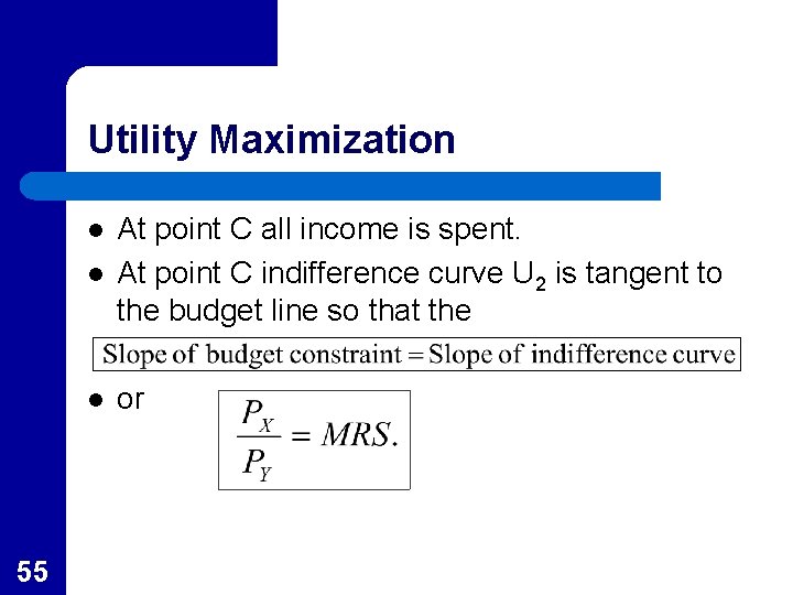
Utility Maximization l At point C all income is spent. At point C indifference curve U 2 is tangent to the budget line so that the l or l 55

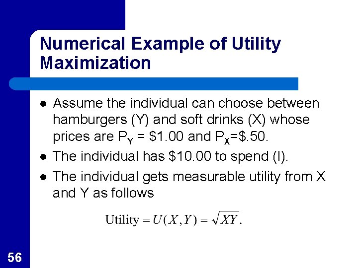
Numerical Example of Utility Maximization l l l 56 Assume the individual can choose between hamburgers (Y) and soft drinks (X) whose prices are PY = $1. 00 and PX=$. 50. The individual has $10. 00 to spend (I). The individual gets measurable utility from X and Y as follows

Using The Model of Choice l l 57 Table 2. 1 lists several possible ways that this person can spend the $10. 00 on hamburgers and soft drinks and the level of utility associated with each choice. The choice of 5 hamburgers and 10 soft drinks yields the most utility as is also demonstrated graphically in Figure 2. 8.

Table 2. 1 58

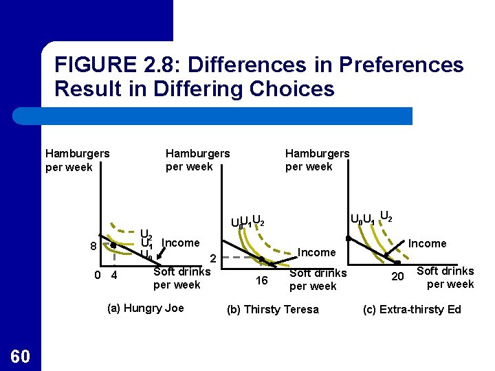
Using the Model of Choice l l 59 The utility maximization model can be used to explain many common observations. Figure 2. 8 shows people with the same income still consume different bundles of goods.

FIGURE 2. 8: Differences in Preferences Result in Differing Choices Hamburgers per week 8 0 4 Hamburgers per week U 2 U 1 Income U 0 2 Soft drinks per week (a) Hungry Joe 60 Hamburgers per week U 0 U 1 U 2 U 0 U 1 U 2 Income 16 Soft drinks per week (b) Thirsty Teresa 20 Soft drinks per week (c) Extra-thirsty Ed

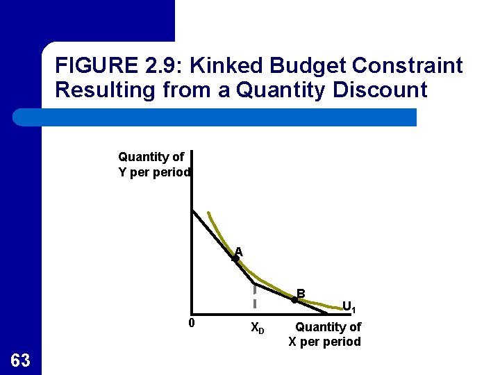
APPLICATION 2. 5: Quantity Discounts and Frequent-Flier Programs l l 61 When consumers receive quantity discounts or have to pay excessive use fees, the budget line is no longer straight. In Figure 2. 9, the consumer pays regular price for good X up to XD but receive a quantity discount beyond that as shown by the flatter budget line after consuming XD.

APPLICATION 2. 5: Quantity Discounts and Frequent-Flier Programs l l 62 Since the consumer is indifferent between points A and B, a slightly larger discount would cause the consumer to reach a higher indifference curve by using the discount. All major airlines use frequent-flier programs that provide such quantity discounts and enable the airlines to gain revenues on seats that otherwise would remain empty.

FIGURE 2. 9: Kinked Budget Constraint Resulting from a Quantity Discount Quantity of Y period A B 0 63 XD U 1 Quantity of X period