CHAPTER 2 Time Domain Representation of Linear Time

CHAPTER 2 Time Domain Representation of Linear Time Invariant (LTI). School of Computer and Communication Engineering, Uni. MAP Nordiana Binti Mohamad Saaid dianams@unimap. edu. my EKT 230 1

2. 0 Time Domain Representation of Linear Time Invariant (LTI) System. 2. 1 2. 2 2. 3 2. 4 2. 5 2. 6 2. 7 2. 8 Introduction. LTI System Properties. Convolution Sum. Convolution Integral. Interconnection of LTI System Properties and Impulse Response. The Step Response. Solving Differential & Difference Equation. 2

2. 1 Introduction. Learning Outcome: Examine several methods for describing the relationship between the input and the output signals of LTI system. (1) Impulse Response. (2) Linear Constant-Coefficient Differential. (3) Block Diagram. 3

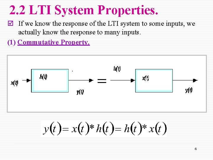
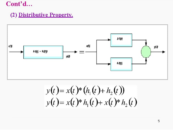
2. 2 LTI System Properties. þ If we know the response of the LTI system to some inputs, we actually know the response to many inputs. (1) Commutative Property. 4

Cont’d… (2) Distributive Property. 5

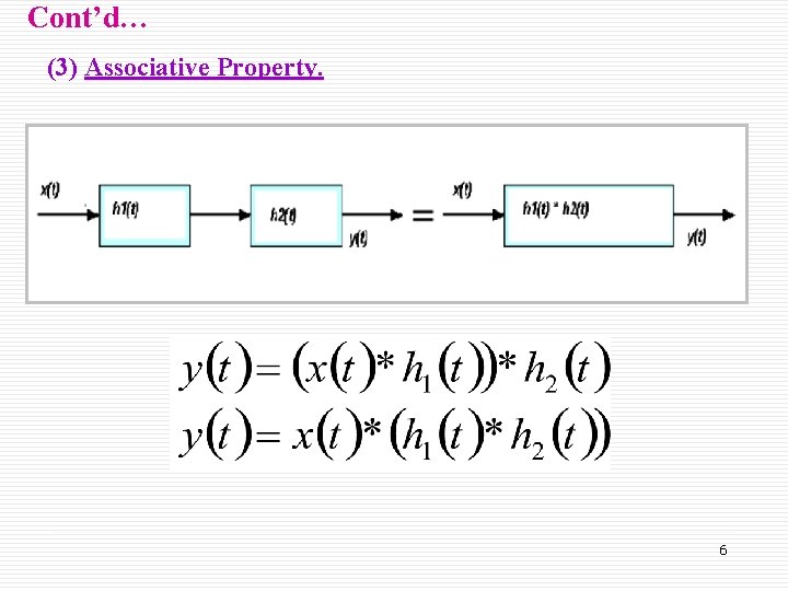
Cont’d… (3) Associative Property. 6

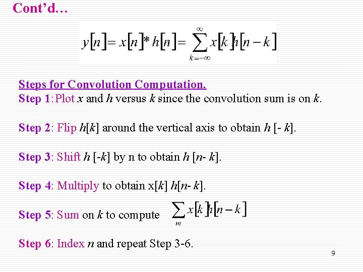
2. 3 Convolution Sum. þ x[n] is a signal as a weighted sum of basic function; time-shift version of the unit impulse signal. x[k] represents a specific value of the signal x[n] at time k. þ The output of the LTI system y[n] is given by a weighted sum of time-shifted impulse response. h[n] is the impulse response of LTI system H. þ The convolution of two discrete-time signals y[n ] and h[n] is denoted as 7

Cont’d… Figure 2. 1: Graphical example illustrating the representation of a signal x[n] as a weighted sum of time-shifted impulses. 8

Cont’d… Steps for Convolution Computation. Step 1: Plot x and h versus k since the convolution sum is on k. 1 Step 2: 2 Flip h[k] around the vertical axis to obtain h [- k]. Step 3: 3 Shift h [-k] by n to obtain h [n- k]. Step 4: 4 Multiply to obtain x[k] h[n- k]. Step 5: 5 Sum on k to compute Step 6: 6 Index n and repeat Step 3 -6. 9

Example 2. 1: Convolution Sum. For the figure below, compute the convolution, y[n]. Figure 2. 2 a: Illustration of the convolution sum. (a) LTI system with impulse response h[n] and input x[n], producing y[n] and yet to be determined. 10

Solution: Figure 2. 2 b: The decomposition of the input x[n] into a weighted sum of time shifted impulses results in an output y[n] given by a weighted sum of time 11 shifted impulse responses.

Example 2. 2: Convolution. The LTI h[n] having an impulse response of and Solution: Details: Explained in class. 12

Example 2. 3: Convolution. The LTI h[n] having an impulse response of and the input Find the convolution of, y[n]=x[n]*h[n]. Solution: ý. 13

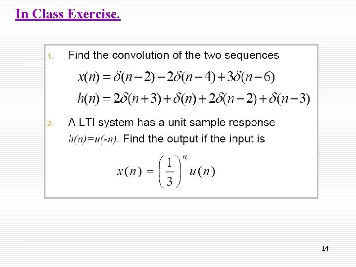
In Class Exercise. 14

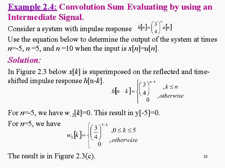
2. 3. 1 Convolution Sum Evaluation Procedure. þ An alternative approach to evaluating the convolution sum. þ Recall, the Convolution Sum is expressed as; define an intermediate signal as; so, þ Time shift n determines the time at which we evaluated the output of the system. þ The above formula is the simplified version of Convolution Sum, 15 where we need to determine one signal wn[k] each time.

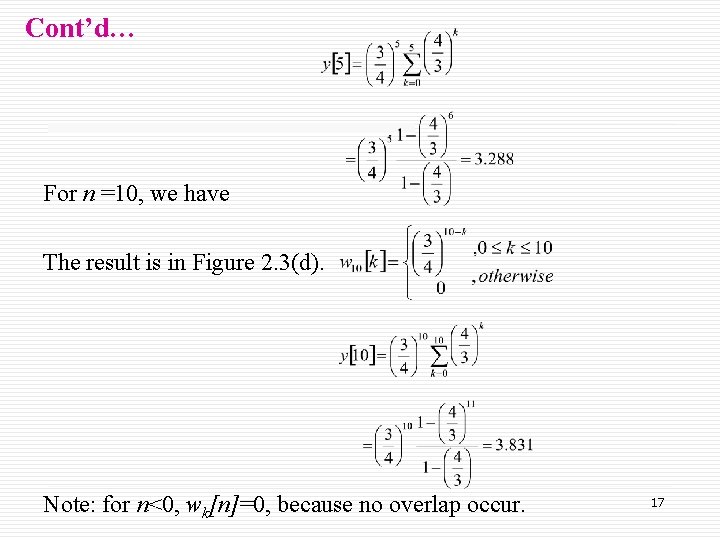
Example 2. 4: Convolution Sum Evaluating by using an Intermediate Signal. Consider a system with impulse response Use the equation below to determine the output of the system at times n=-5, n =5, and n =10 when the input is x[n]=u[n]. Solution: In Figure 2. 3 below x[k] is superimposed on the reflected and timeshifted impulse response h[n-k]. For n=-5, we have w-5[k]=0. This result in y[-5]=0. For n=5, we have The result is in Figure 2. 3(c). 16

Cont’d… For n =10, we have The result is in Figure 2. 3(d). Note: for n<0, wk[n]=0, because no overlap occur. 17

Cont’d… Figure 2. 3: (a) The input signal x[k] above the reflected and time-shifted impulse response h[n – k], depicted as a function of k. (b) The product signal w 5[k] used to evaluate y [– 5]. (c) The product signal w 5[k] used to evaluate y[5]. (d) The product signal w 10[k] used to evaluate y[10]. 18

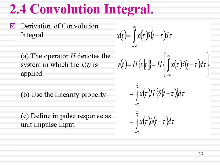
2. 4 Convolution Integral. þ Derivation of Convolution Integral. (a) The operator H denotes the system in which the x(t) is applied. (b) Use the linearity property. (c) Define impulse response as unit impulse input. 19

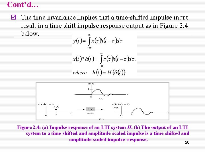
Cont’d… þ The time invariance implies that a time-shifted impulse input result in a time shift impulse response output as in Figure 2. 4 below. Figure 2. 4: (a) Impulse response of an LTI system H. (b) The output of an LTI system to a time-shifted and amplitude-scaled impulse is a time-shifted and amplitude-scaled impulse response. 20

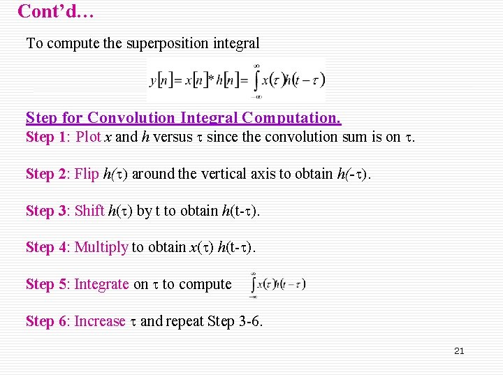
Cont’d… To compute the superposition integral Step for Convolution Integral Computation. Step 1: 1 Plot x and h versus t since the convolution sum is on t. Step 2: 2 Flip h(t) around the vertical axis to obtain h(-t). Step 3: 3 Shift h(t) by t to obtain h(t-t). Step 4: 4 Multiply to obtain x(t) h(t-t). Step 5: 5 Integrate on t to compute Step 6: 6 Increase t and repeat Step 3 -6. 21

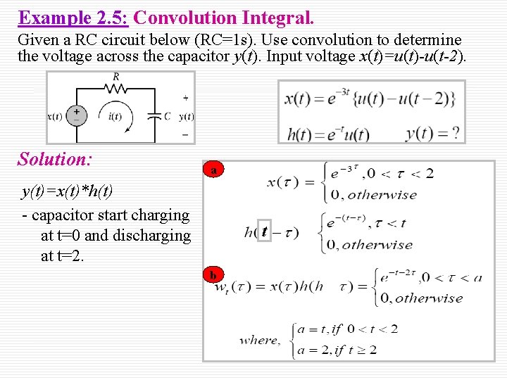
Example 2. 5: Convolution Integral. Given a RC circuit below (RC=1 s). Use convolution to determine the voltage across the capacitor y(t). Input voltage x(t)=u(t)-u(t-2). Solution: a y(t)=x(t)*h(t) - capacitor start charging at t=0 and discharging at t=2. t b 22

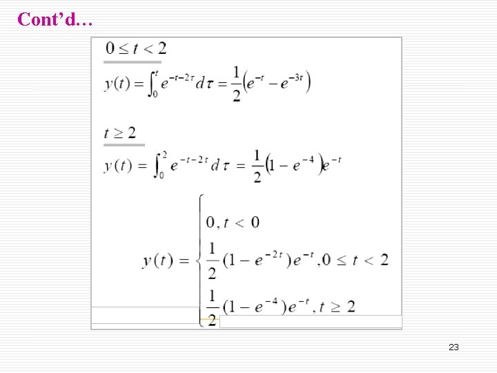
Cont’d… 23

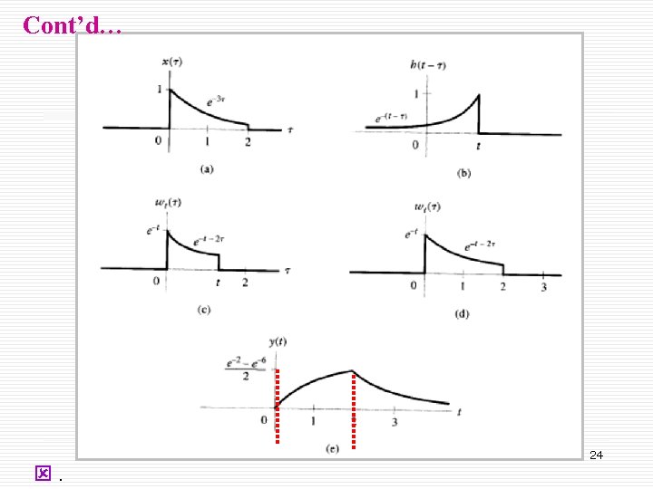
Cont’d… ý. 24

2. 5 Interconnection of LTI System. þ The objective of this section is to develop the relationship between the impulse response of an interconnection of LTI systems and impulse response of the constituent systems. 2. 5. 1 Parallel Connection of LTI System. 2. 5. 2 Cascade Connection of LTI System. 25

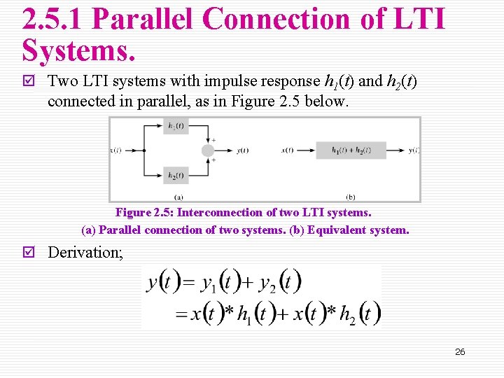
2. 5. 1 Parallel Connection of LTI Systems. þ Two LTI systems with impulse response h 1(t) and h 2(t) connected in parallel, as in Figure 2. 5 below. Figure 2. 5: Interconnection of two LTI systems. (a) Parallel connection of two systems. (b) Equivalent system. þ Derivation; 26

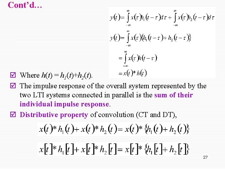
Cont’d… þ Where h(t) = h 1(t)+h 2(t). þ The impulse response of the overall system represented by the two LTI systems connected in parallel is the sum of their individual impulse response þ Distributive property of convolution (CT and DT), 27

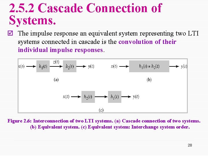
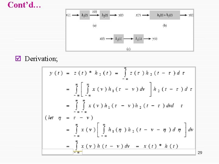
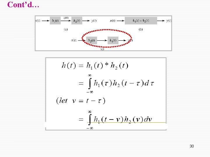
2. 5. 2 Cascade Connection of Systems. þ The impulse response an equivalent system representing two LTI systems connected in cascade is the convolution of their individual impulse responses Figure 2. 6: Interconnection of two LTI systems. (a) Cascade connection of two systems. (b) Equivalent system. (c) Equivalent system: Interchange system order. 28

Cont’d… þ Derivation; 29

Cont’d… 30

Cont’d… 31

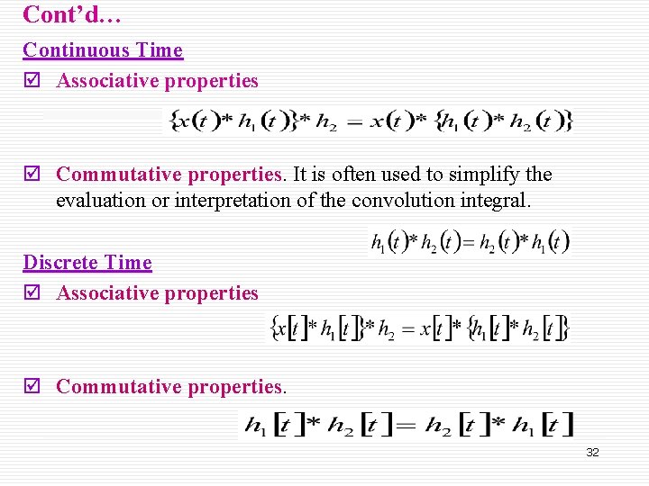
Cont’d… Continuous Time þ Associative properties þ Commutative properties. It is often used to simplify the evaluation or interpretation of the convolution integral. Discrete Time þ Associative properties þ Commutative properties. 32

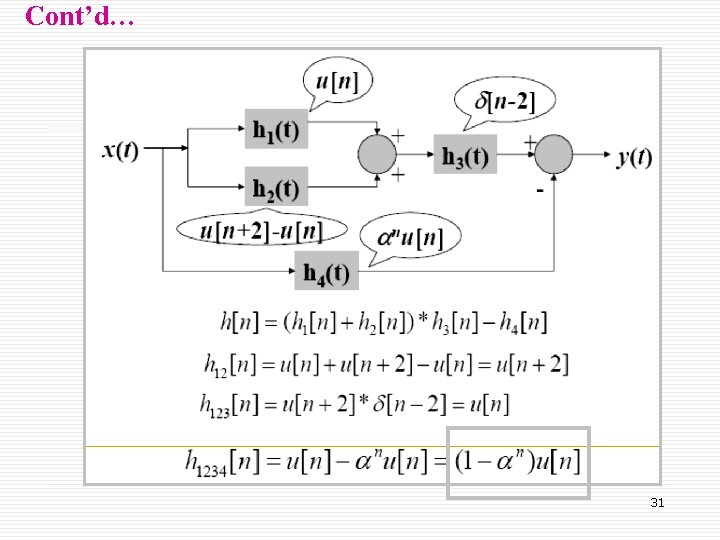
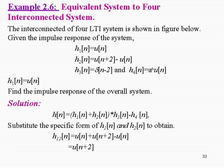
Example 2. 6: Equivalent System to Four Interconnected System. The interconnected of four LTI system is shown in figure below. Given the impulse response of the system, h 1[n]=u[n] h 2[n]=u[n+2]- u[n] h 3[n]=d[n-2] and h 4[n]=anu[n] h 1[n]=u[n] Find the impulse response of the overall system. Solution: h[n]=(h 1[n]+h 2[n])*h 3[n]-h 4 [n], Substitute the specific form of h 1[n] and h 2[n] to obtain. h 12[n]=u[n]+u[n+2]-u[n] =u[n+2] 33

Cont’d… Convolving h 12[n] with h 3[n]. h 123 [n]= u[n]+u[n+2]*d[n] = u[n] Finally, we sum h 123[n] and -h 4[n] to obtain the overall impulse response: h[n]= {1 -an}u[n]. Figure 2. 7 : Interconnection of systems. ý. 34

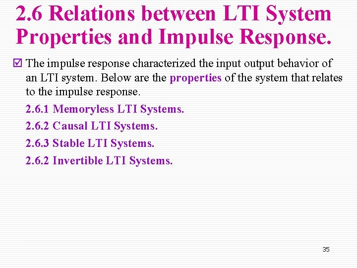
2. 6 Relations between LTI System Properties and Impulse Response. þ The impulse response characterized the input output behavior of an LTI system. Below are the properties of the system that relates to the impulse response. 2. 6. 1 Memoryless LTI Systems. 2. 6. 2 Causal LTI Systems. 2. 6. 3 Stable LTI Systems. 2. 6. 2 Invertible LTI Systems. 35

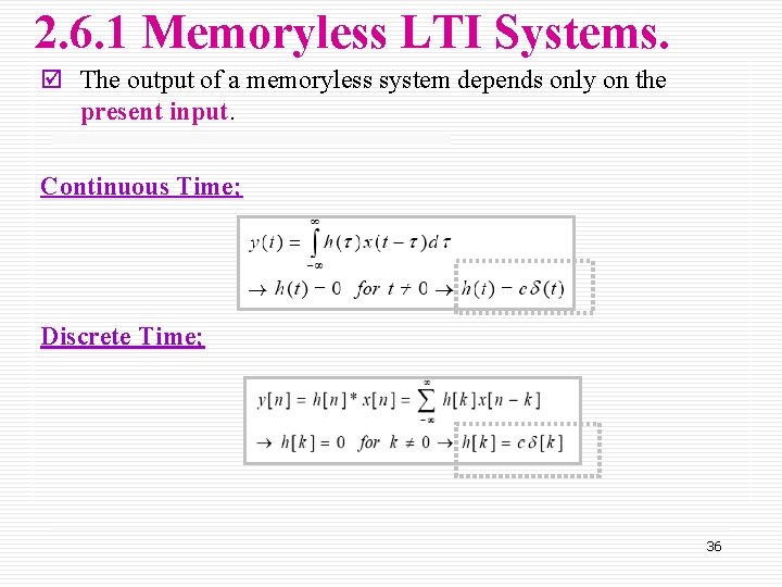
2. 6. 1 Memoryless LTI Systems. þ The output of a memoryless system depends only on the present input. Continuous Time; Discrete Time; 36

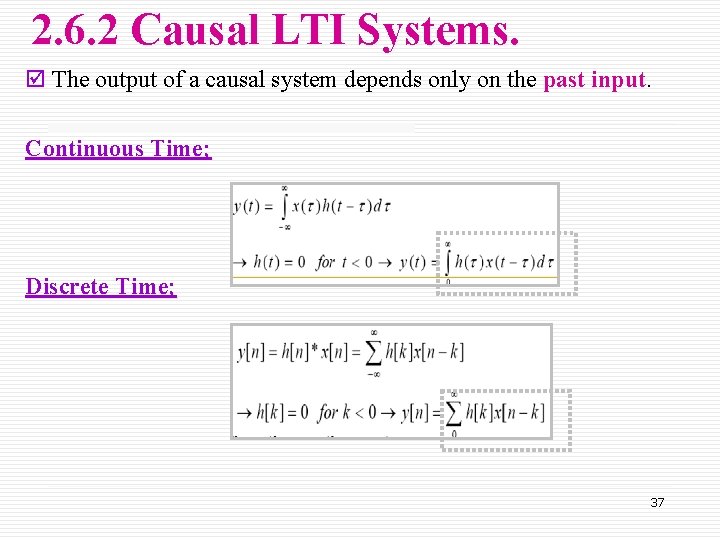
2. 6. 2 Causal LTI Systems. þ The output of a causal system depends only on the past input. Continuous Time; Discrete Time; 37

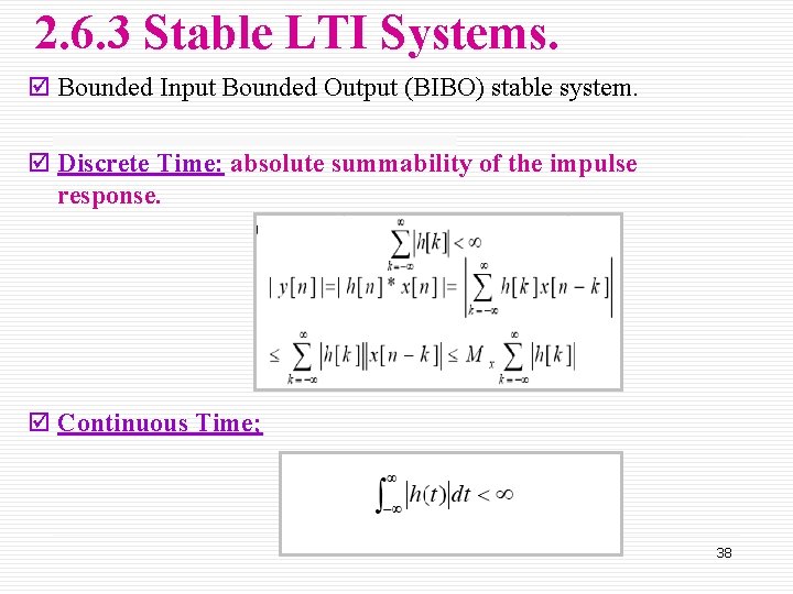
2. 6. 3 Stable LTI Systems. þ Bounded Input Bounded Output (BIBO) stable system. þ Discrete Time: absolute summability of the impulse response. þ Continuous Time; 38

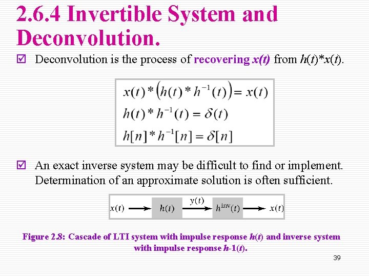
2. 6. 4 Invertible System and Deconvolution. þ Deconvolution is the process of recovering x(t) from h(t)*x(t). þ An exact inverse system may be difficult to find or implement. Determination of an approximate solution is often sufficient. Figure 2. 8: Cascade of LTI system with impulse response h(t) and inverse system with impulse response h-1(t). 39

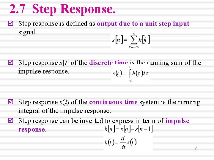
2. 7 Step Response. þ Step response is defined as output due to a unit step input signal. þ Step response s[t] of the discrete time is the running sum of the impulse response. þ Step response s(t) of the continuous time system is the running integral of the impulse response. þ Step response can be inverted to express in term of impulse response. 40

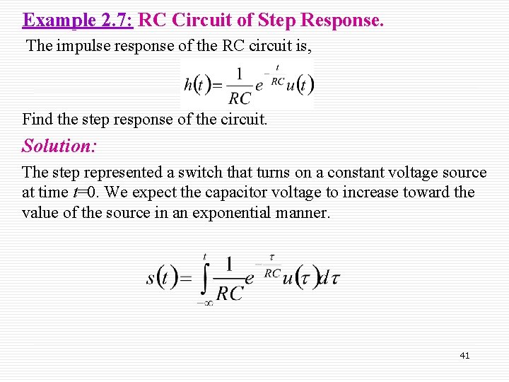
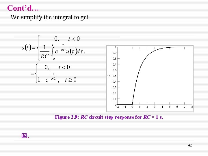
Example 2. 7: RC Circuit of Step Response. The impulse response of the RC circuit is, Find the step response of the circuit. Solution: The step represented a switch that turns on a constant voltage source at time t=0. We expect the capacitor voltage to increase toward the value of the source in an exponential manner. 41

Cont’d… We simplify the integral to get Figure 2. 9: RC circuit step response for RC = 1 s. ý. 42

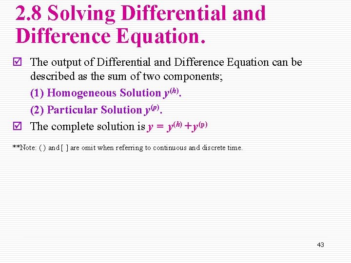
2. 8 Solving Differential and Difference Equation. þ The output of Differential and Difference Equation can be described as the sum of two components; (1) Homogeneous Solution y(h). (2) Particular Solution y(p). þ The complete solution is y = y(h) + y(p) **Note: ( ) and [ ] are omit when referring to continuous and discrete time. 43

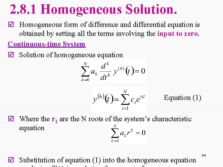
2. 8. 1 Homogeneous Solution. þ Homogeneous form of difference and differential equation is obtained by setting all the terms involving the input to zero. Continuous-time System þ Solution of homogeneous equation Equation (1) þ Where the r 1 are the N roots of the system’s characteristic equation þ Substitution of equation (1) into the homogeneous equation 44

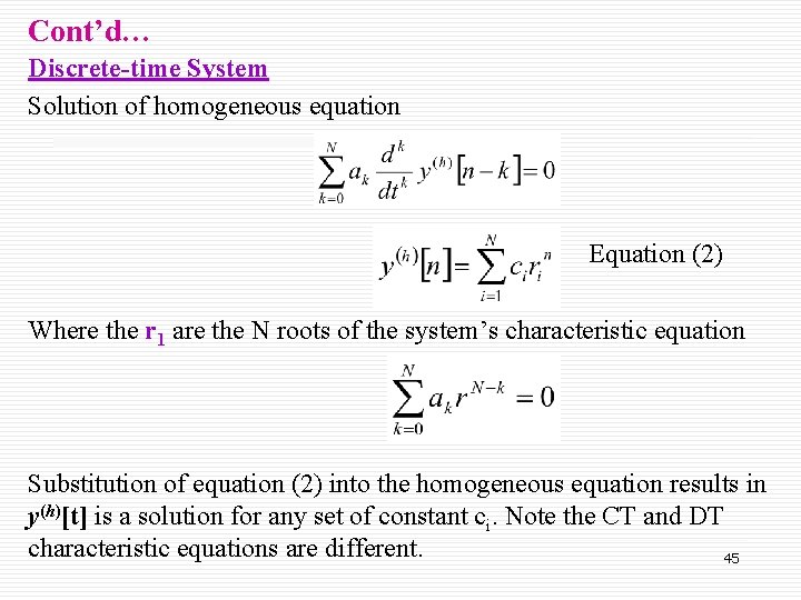
Cont’d… Discrete-time System Solution of homogeneous equation Equation (2) Where the r 1 are the N roots of the system’s characteristic equation Substitution of equation (2) into the homogeneous equation results in y(h)[t] is a solution for any set of constant ci. Note the CT and DT characteristic equations are different. 45

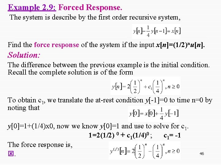
Example 2. 9: Forced Response. The system is describe by the first order recursive system, Find the force response of the system if the input x[n]=(1/2)nu[n]. Solution: The difference between the previous example is the initial condition. Recall the complete solution is of the form To obtain c 1, we translate the at-rest condition y[-1]=0 to time n=0 by noting that y[0]=1+(1/4)x 0, now we know y[0]=1 and use to solve for c 1. 1=2(1/2) 0 + c 1(1/4)0 ; c 1= -1 The force response is, ý. 46

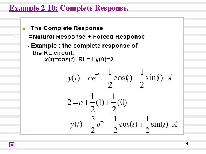
Example 2. 10: Complete Response. ý. 47

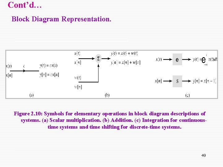
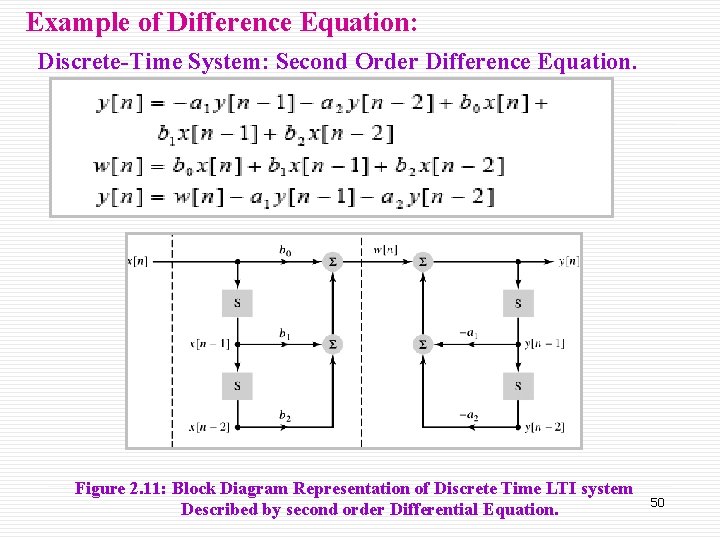
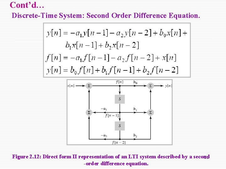
Block Diagram Representation. þ Block diagram is an interconnection of elementary operations that act on the input signal. þ A more detailed representation of the system than the impulse response or differential (difference) equation description since it describes how the system’s internal computations or operations are ordered. þ Block diagram representations consists of an interconnection of three elementary operations on signals; (1) Scalar Multiplication. (2) Addition. (3) Integration for continuous-time LTI system. 48

Cont’d… Block Diagram Representation. Figure 2. 10: Symbols for elementary operations in block diagram descriptions of systems. (a) Scalar multiplication. (b) Addition. (c) Integration for continuoustime systems and time shifting for discrete-time systems. 49

Example of Difference Equation: Discrete-Time System: Second Order Difference Equation. Figure 2. 11: Block Diagram Representation of Discrete Time LTI system Described by second order Differential Equation. 50

Cont’d… Discrete-Time System: Second Order Difference Equation. Figure 2. 12: Direct form II representation of an LTI system described by a second 51 -order difference equation.