Chapter 2 The Labor Market Definitions Facts and

Chapter 2. The Labor Market: Definitions, Facts, and Trends.

The Labor Market: Definitions, Facts, and Trends • The Labor Force and Unemployment • The Earnings of Labor How the Labor Market Works • The Demand for Labor • The Supply of Labor • The Determination of the Wage • Rents Applications of the Theory
 Civilian noninstitutional population. – persons 16 years of age")
Labor Force Measures • (Adult) Civilian noninstitutional population. – persons 16 years of age and older – residing in the 50 States & DC – not inmates of institutions (e. g. , penal and mental facilities, homes for the aged), – not on active duty in the Armed Forces.

Labor Force Measures • Employed persons. – during the reference week, • did any work at all (at least 1 hour) as paid employees, • worked in their own business, profession, or on their own farm, • or worked 15 hours or more as unpaid workers in an enterprise operated by a member of the family, • all those who were not working but who had jobs or businesses from which they were temporarily absent (vacation, sick)

Labor Force Measures • Unemployed persons. – no employment during the reference week, – available for work, except for temporary illness, and made specific efforts to find employment some time during the 4 -weekperiod ending with the reference week. – Persons who were waiting to be recalled to a job from which they had been laid off need not have been looking for work to be classified as unemployed.

Labor Force Measures • Labor force. employed + unemployed • Unemployment rate. Unemployed / Labor Force • Labor Force Participation rate. Labor Force / Civ. Non. Inst. Pop • Employment-population ratio. Employed/ Civ. Noninst. Pop. • Historical Data – (Table B 35 from Econ. Report)
 Civilian")
1990/2014 Data Adult Civilian Noninstiutionalized Population (189. 164 m / 248. 023 m) Civilian Labor Force (125. 840 m / 156. 023 m. ) Employed (118. 793 m. / 146. 352 m. ) Not in labor force (63. 324 m / 92. 001 m) Unemployed (7. 047 m / 9. 671 m. )

Labor force measures 1990 Unemployment rate Labor force participation rate Employment rate 2014

Labor force measures 1990 2014 Unemployment rate 5. 6% 6. 2% Civilian Labor force participation rate Employmentpopulation ratio (employment rate) 66. 5% 62. 9% 62. 8% 59. 0%

• Start with ØU=10 million, E=90 million, CNIP=200 million • What would happen to unempl rate, lfpr, and empl rate if – 10 million people out of labor force begin looking for work and 6 million find jobs. – 1 million unemployed people become “discourage” and quit looking for work? – 1 million unemployed people find new jobs? – 1 million employed people lose jobs and. 5 million choose to retire while the other. 5 million begin search for new jobs.

1. Between 2010 & 2011, unemployment rate and employment rate both fell. How is this possible? 2. Based on the growth in Civilian Non-institutional Population between 2012 and 2013, how many jobs would have to be added during 2013 to keep the unemployment rate at 8. 1% if LFPR a. stayed at 2013 level (63. 2%)? b. rises to 2012 level (63. 7%)? c. rises to level prior to recession (66. 0%)?
 LFP UR")
Estimating Required Job Growth for Constant Unemployment Rate CNIP (in 1000 s) LFP UR CLF (in 1000 s) Employed (in 1000 s) 2012 243, 284 63. 70% 8. 10% 154, 975 142, 468 2013 245, 679 63. 25% 7. 40% 155, 389 143, 929 + Assumed LFP Jobs required Annual Monthly for 8. 1% Change in CLF in 2013 based unemployment jobs relative on LFP rate to 2012 (in 1000 s) 63. 2% 155, 269 142, 692 224 19 63. 7% 156, 498 143, 821 1, 353 113 66. 0% 162, 148 149, 014 6, 546 Article on jobs needed per month
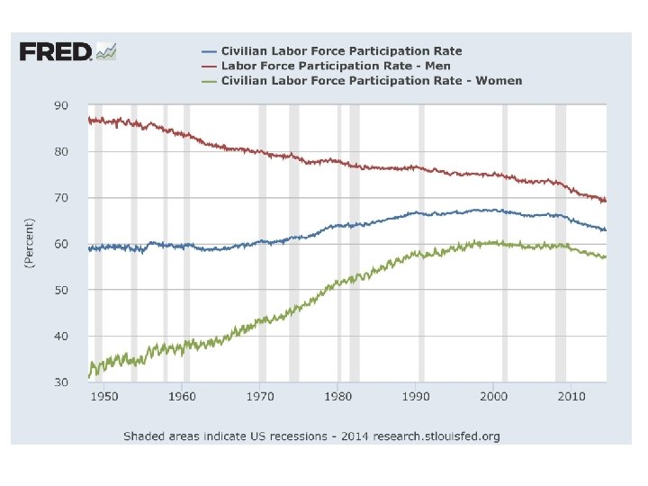
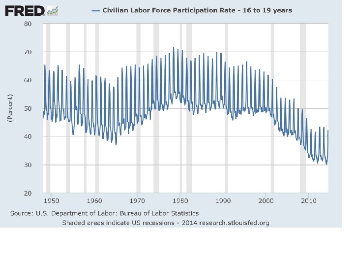
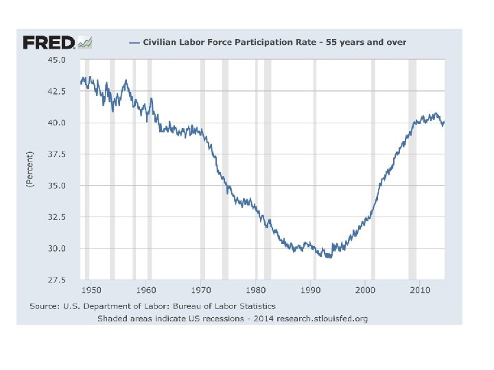

Variation in unemployment rates • Employment Situation from bls. gov – Sex – Age – Education • Why is there a correlation between these characteristics and unemployment rates? • Unemployment and employment rates by state.

Labor Earnings • Wage rate X hours worked =Earnings • Earnings + Benefits = Total Compensation • Total compensation + unearned (nonlabor) income = Total Income

Earnings Measures

Real versus Nominal Wages. • CPIt = • Real Waget = • Nominal Wage represents earnings in current dollars. • Real Wage represents earnings in constant (base year) dollars.

Real versus Nominal Wages. • Issues with Indexing – The bundle • Varies across people/time. • Evidence that CPI over-states growth in cost of living by 1 to 1. 5 percent per year. – Quality of goods – Substitution effects • Point in time adjustments versus across time – Comparable salary in city j = salary in city k * city j cpi city k cpi
 • If a person")
Real versus Nominal Wages. • CPI data (available from BLS) • If a person earned $8 per hour in 1980, what would yield the equivalent purchasing power in 2014? • If a person’s nominal wage rose from $10 per hour in 2000 to $15 per hour by 2014, what happened to her real wage (in 1982 -84 dollars)?

Using the CPI to convert present values into past values and vice versa – see row 4 for 1980, 1990, and 2012: Computations 1980 1990 (0. 99)31 x$19. 09 ≈ $13. 97 (0. 99)21 x $17. 92 ≈ $14. 51 2012 Row 3: Row 4: Row 5: (Adjustment in real wages by 1%) $19. 77
 • If a person moved")
Earnings Measures • Cost of Living by City (ACCRA) • If a person moved from Cincinnati to San Francisco and his earnings rose from $50, 000 to $70, 000, did his real earnings rise or fall? • What are some of the problems with the Cinci/San Francisco comparison?
 – scale effect – substitution")
Labor Demand • Changes in wages (move along D-curve) – scale effect – substitution effect • Changes in other factors (shift D-curve) – demand for product • scale effect, no substitution effect – supply of other inputs (e. g. capital) • scale effect and substitution effect

Labor Demand • Market, Industry, and Firm Demand. – different ways of measuring labor demand. • Long run versus short run demand. – Subst. effects tend to be larger in the LR, labor demand more elastic in the long run.

Labor Supply • Labor supply curve. – Market supply curve: upward sloping. – Firm supply curve: horizontal in competitive market. • Factors shifting labor supply: – population. – alternative opportunities (other employment, nonemployment) – taxes – non-pecuniary aspects of job (fringes, risk, night shifts, etc. )

Labor Market Equilibrium • If wage is below equilibrium: shortage. • If wage is above equilibrium: surplus (unemployment). • Shortages put upward pressure on wages. Surpluses put downward pressure on wages. • Workers receive “economic rents” - Difference between what they are paid and minimum they are willing to accept. - Area between wage rate and labor supply curve

Labor Market Equilibrium • Effect of – Increased population – Increased tax on employers – Increased tax on employees – Cheaper capital – Cheaper imports (consumer versus intermediate goods) – Increased demand for product
- Slides: 29