Chapter 2 System Models Time Domain 1 Model

Chapter 2 System Models – Time Domain 1

Model of a System • Mathematical equation that describes the relationship between input x(t) or x[n] and the output y(t) or y[n]. • Drawing or diagram that illustrates the input – output relationship • Words that define the inputs, outputs, and their relationship. 2

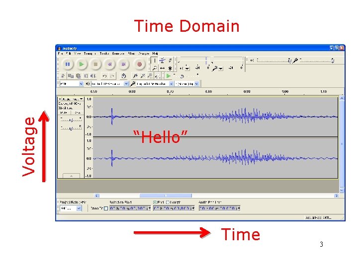
Voltage Time Domain “Hello” Time 3

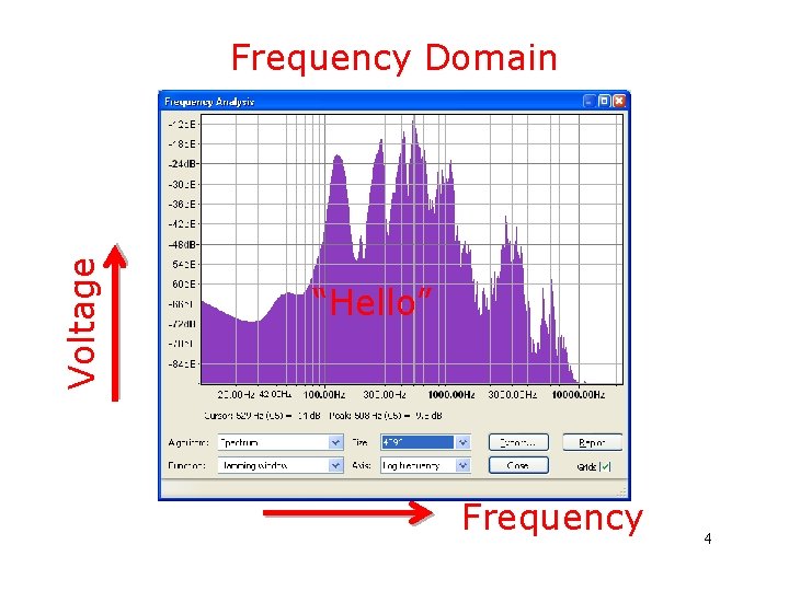
Voltage Frequency Domain “Hello” Frequency 4

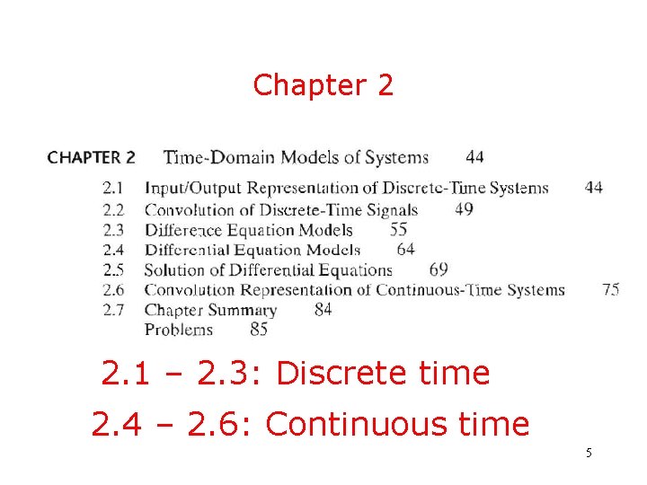
Chapter 2 2. 1 – 2. 3: Discrete time 2. 4 – 2. 6: Continuous time 5

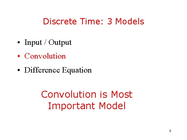
Discrete Time: 3 Models • Input / Output • Convolution • Difference Equation Convolution is Most Important Model 6

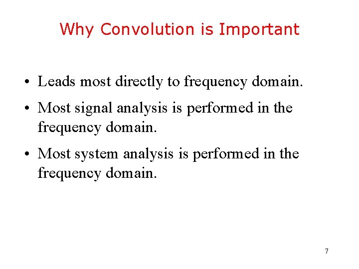
Why Convolution is Important • Leads most directly to frequency domain. • Most signal analysis is performed in the frequency domain. • Most system analysis is performed in the frequency domain. 7

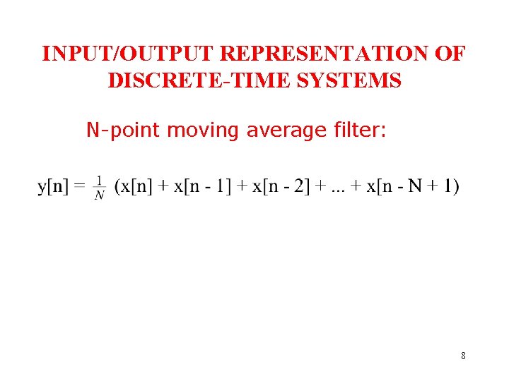
INPUT/OUTPUT REPRESENTATION OF DISCRETE-TIME SYSTEMS N-point moving average filter: 8

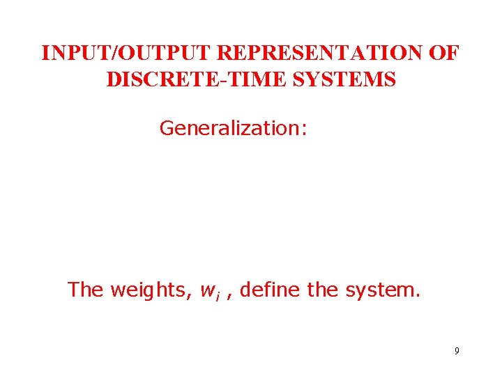
INPUT/OUTPUT REPRESENTATION OF DISCRETE-TIME SYSTEMS Generalization: The weights, wi , define the system. 9

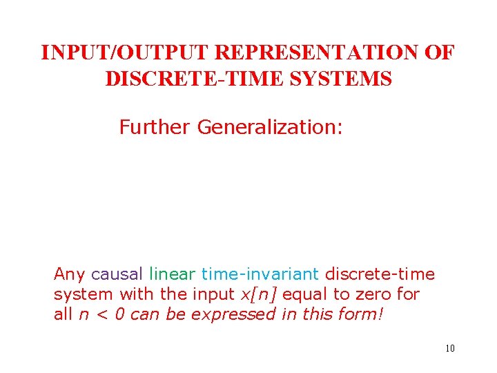
INPUT/OUTPUT REPRESENTATION OF DISCRETE-TIME SYSTEMS Further Generalization: Any causal linear time-invariant discrete-time system with the input x[n] equal to zero for all n < 0 can be expressed in this form! 10

UNIT-PULSE RESPONSE Denote by h[n] Set x[n] = δ[n] 11

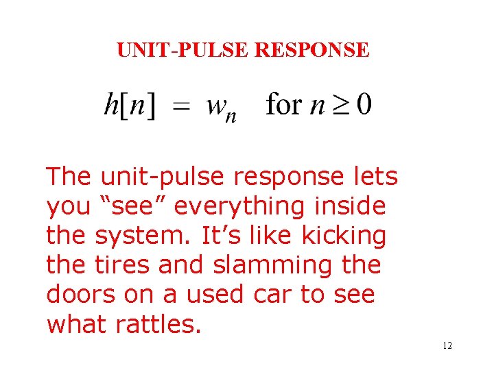
UNIT-PULSE RESPONSE The unit-pulse response lets you “see” everything inside the system. It’s like kicking the tires and slamming the doors on a used car to see what rattles. 12

CONVOLUTION REPRESENTATION Rewriting the I/O equation using h[n] yields CONVOLUTION 13

CONVOLUTION EXAMPLE >> >> x=[1 0 0 0]; % input unit pulse h=[1 2 3 2 1]; % unit pulse response y=conv(x, h); % output y y= 1 2 3 2 1 0 0 0 >> More about computing convolution later… 14

DIFFERENCE EQUATION MODEL (Sect. 2. 3) Nth-Order Input/Output Difference Equation: Present output, y[n], depends on previous inputs and outputs, and present input, x[n]. Solve recursively, or find a closed-form solution. 15

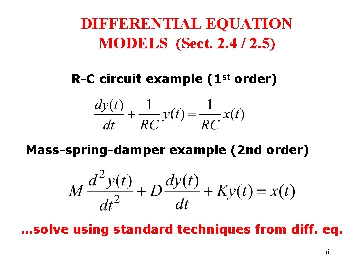
DIFFERENTIAL EQUATION MODELS (Sect. 2. 4 / 2. 5) R-C circuit example (1 st order) Mass-spring-damper example (2 nd order) …solve using standard techniques from diff. eq. 16