Chapter 2 Supply and Demand DEMAND Quantity demanded

Chapter 2 Supply and Demand

DEMAND –Quantity demanded is the amount of a good, service, or resource that people are willing and able to buy during a specified period at a specified price. –The quantity demanded is an amount per unit of time. For example, the amount per day or per month.

DEMAND <The Law of Demand – Other things remaining the same, • If the price of the good rises, the quantity demanded of that good decreases. • If the price of the good falls, the quantity demanded of that good increases.

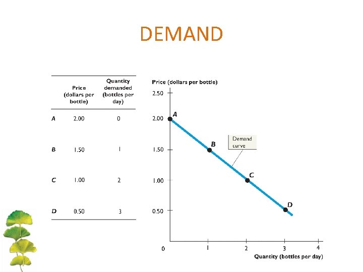
DEMAND <Demand Schedule and Demand Curve –Demand is the relationship between the quantity demanded and the price of a good when all other influences on buying plans remain the same. –Demand is illustrated by a demand schedule and a demand curve.

DEMAND –Demand schedule is a list of the quantities demanded at each different price when all the other influences on buying plans remain the same. –Demand curve is a graph of the relationship between the quantity demanded of a good and its price when all other influences on buying plans remain the same.

DEMAND

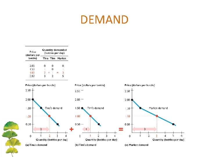
DEMAND <Individual Demand Market Demand –Market demand is the sum of the demands of all the buyers in a market. –The market demand curve is the horizontal sum of the demand curves of all buyers in the market.

DEMAND

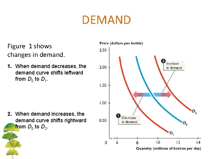
DEMAND <Changes in Demand – Change in demand is a change in the quantity that people plan to buy when any influence other than the price of the good changes. – A change in demand means that there is a new demand schedule and a new demand curve.

DEMAND Figure 1 shows changes in demand. 1. When demand decreases, the demand curve shifts leftward from D 0 to D 1. 2. When demand increases, the demand curve shifts rightward from D 0 to D 2.

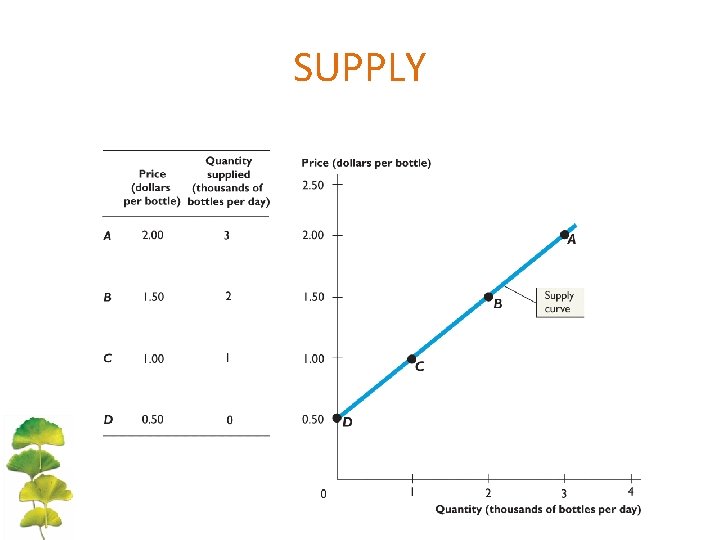
SUPPLY Quantity supplied is the amount of a good, service, or resource that people are willing and able to sell during a specified period at a specified price. < The Law of Supply Other things remaining the same, • If the price of a good rises, the quantity supplied that good increases. of • If the price of a good falls, the quantity supplied of that good decreases.

SUPPLY <Supply Schedule and Supply Curve –Supply is the relationship between the quantity supplied of a good and the price of the good when all other influences on selling plans remain the same. –Supply is illustrated by a supply schedule and a supply curve.

SUPPLY A supply schedule is a list of the quantities supplied at each different price when all other influences on selling plans remain the same. A supply curve is a graph of the relationship between the quantity supplied and the price of the good when all other influences on selling plans remain the same.

SUPPLY

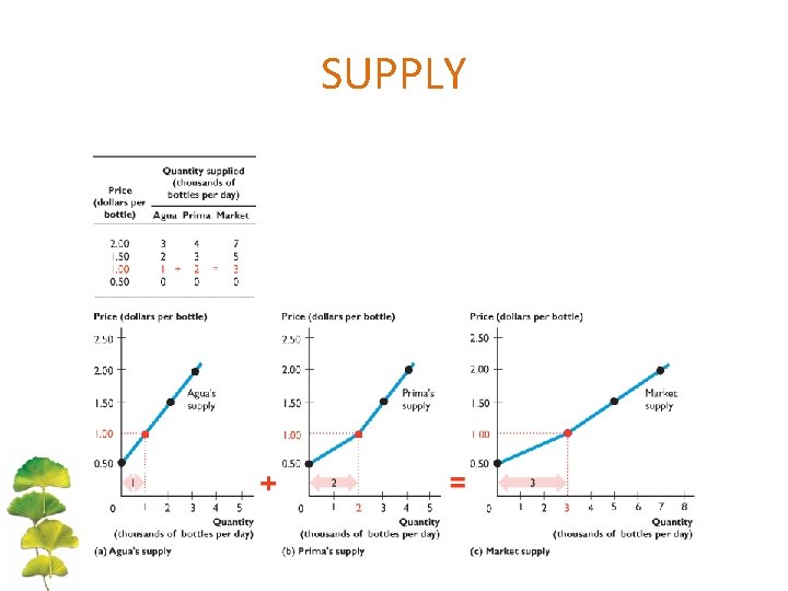
SUPPLY <Individual Supply and Market Supply – Market supply is the sum of the supplies of all sellers in a market. – The market supply curve is the horizontal sum of the supply curves of all the sellers in the market.

SUPPLY

SUPPLY <Changes in Supply – A change in supply is a change in the quantity that suppliers plan to sell when any influence on selling plans other than the price of the good changes. – A change in supply means that there is a new supply schedule and a new supply curve.

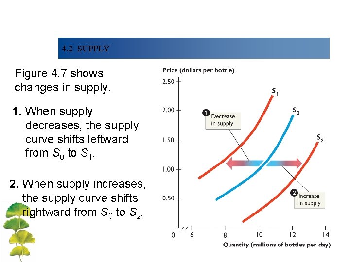
4. 2 SUPPLY Figure 4. 7 shows changes in supply. 1. When supply decreases, the supply curve shifts leftward from S 0 to S 1. 2. When supply increases, the supply curve shifts rightward from S 0 to S 2.

MARKET EQUILIBRIUM Market equilibrium occurs when the quantity demanded equals the quantity supplied. At market equilibrium, buyers’ and sellers’ plans are consistent. Equilibrium price is the price at which the quantity demanded equals the quantity supplied. Equilibrium quantity is the quantity bought and sold at the equilibrium price.

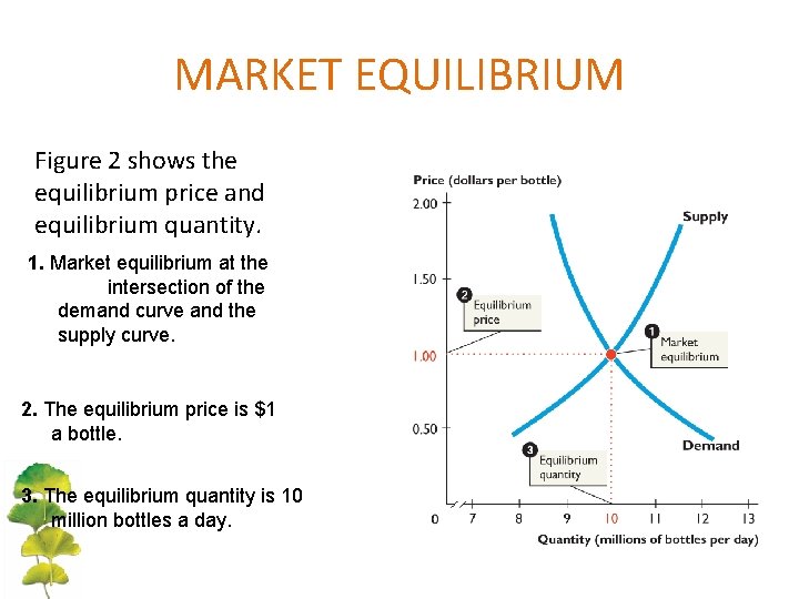
MARKET EQUILIBRIUM Figure 2 shows the equilibrium price and equilibrium quantity. 1. Market equilibrium at the intersection of the demand curve and the supply curve. 2. The equilibrium price is $1 a bottle. 3. The equilibrium quantity is 10 million bottles a day.

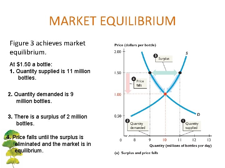
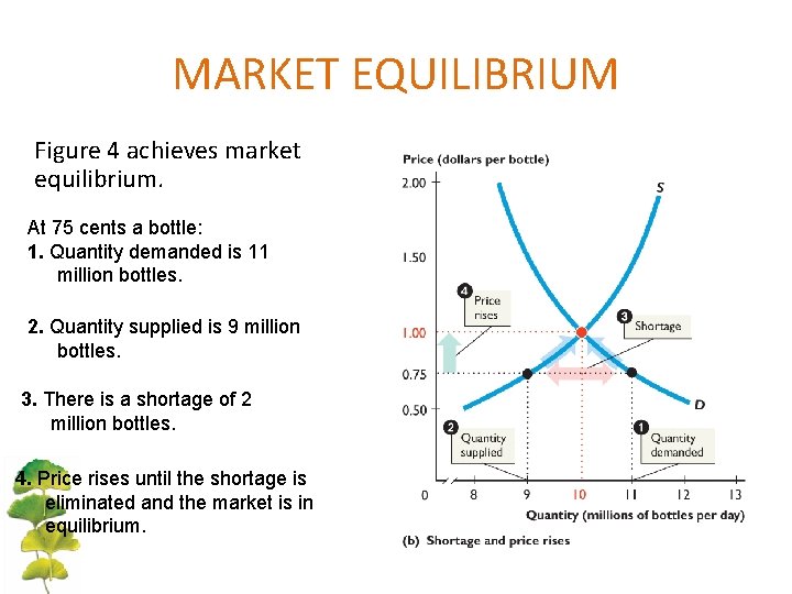
MARKET EQUILIBRIUM • Price: A Market’s Automatic Regulator –Law of market forces • When there is a shortage, the price rises. • When there is a surplus, the price falls. –Shortage occurs when the quantity demanded exceeds the quantity supplied. –Surplus occurs when the quantity supplied exceeds the quantity demanded.

MARKET EQUILIBRIUM Figure 3 achieves market equilibrium. At $1. 50 a bottle: 1. Quantity supplied is 11 million bottles. 2. Quantity demanded is 9 million bottles. 3. There is a surplus of 2 million bottles. 4. Price falls until the surplus is eliminated and the market is in equilibrium.

MARKET EQUILIBRIUM Figure 4 achieves market equilibrium. At 75 cents a bottle: 1. Quantity demanded is 11 million bottles. 2. Quantity supplied is 9 million bottles. 3. There is a shortage of 2 million bottles. 4. Price rises until the shortage is eliminated and the market is in equilibrium.

DETERMINANTS OF SUPPLY AND DEMAND Supply and demand analysis is useful not only for the normative insight it offers into questions of public policy but also for a rich variety of descriptive purposes. Most important, it predicts how equilibrium prices and quantities will respond to changes in market forces. Because supply and demand curves intersect to determine equilibrium prices and quantities, anything that shifts these curves will alter equilibrium values in a predictable way. © 2015 Mc. Graw-Hill Education. All Rights Reserved. 33

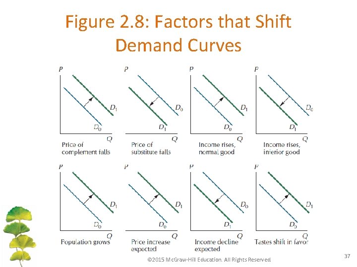
Factors the Shift the Demand Curve • Incomes – Normal goods: the quantity demanded at any price rises with income. – Inferior goods: the quantity demanded at any price falls with income. • Tastes vary across people and over time. In Western societies, culture instills a taste for sitting on padded furniture, whereas in many Eastern societies, people are conditioned to favor sitting cross-legged on the floor. The demand for armchairs thus tends to be larger in the West than in the East. © 2015 Mc. Graw-Hill Education. All Rights Reserved. 34

• Price of Substitutes and Complements - an increase in the price of one good decreases demand for the other good. Substitutes - an increase in the price of one will tend to increase the demand for the other. • Expectations about future income and price levels also affect current purchase decisions. For example, someone who expects higher future income is likely to spend more today than an otherwise identical person who expects lower future income. (After all, with higher expected future income, the need to save diminishes. ) Similarly, people will often accelerate their current purchases of goods whose prices are expected to rise in the months to come. © 2015 Mc. Graw-Hill Education. All Rights Reserved. 35

• Population In general, the number of people who buy a product grows as the number of potential buyers grows. Thus, in cities with growing populations, the demand for housing increases from year to year, whereas it tends to fall in cities with declining populations. © 2015 Mc. Graw-Hill Education. All Rights Reserved. 36

Figure 2. 8: Factors that Shift Demand Curves © 2015 Mc. Graw-Hill Education. All Rights Reserved. 37

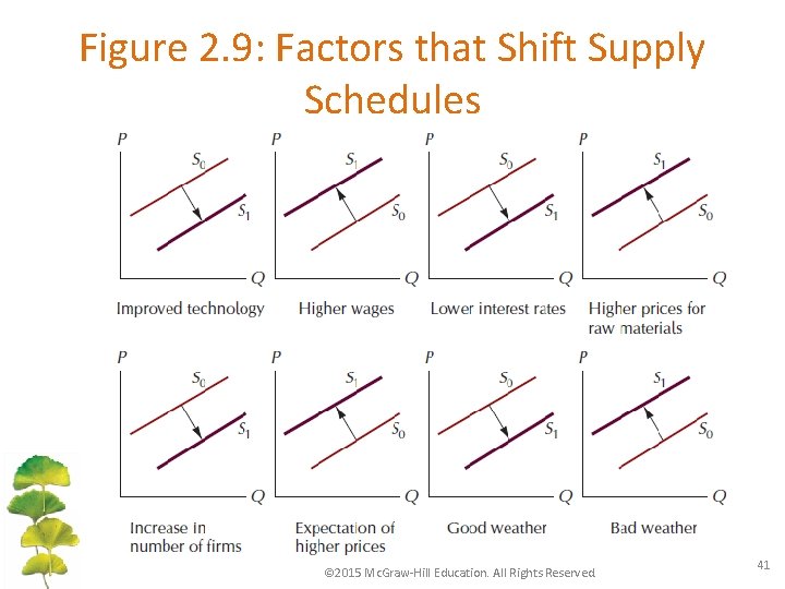
DETERMINANTS OF SUPPLY Factors the Shift the Supply Curve • • • Technology Factor Prices The Number of Suppliers Expectations Weather © 2015 Mc. Graw-Hill Education. All Rights Reserved. 38

Technology The amount suppliers are willing to offer at any price depends primarily on their costs of production. These costs, in turn, are closely linked to technology. For instance, the discovery of a more efficient lobster trap will reduce the cost of harvesting lobsters, which results in a rightward shift in the supply schedule. Factor Prices A supplier’s costs also depend on the payment it must make to its factors of production: labor, capital, and so on. If the price of lobster boats rises, or if the wage paid to lobstermen goes up, the supply schedule for lobsters shifts to the left. © 2015 Mc. Graw-Hill Education. All Rights Reserved. 39

The Number of Suppliers The more firms that can supply a good, the greater will be the quantity supplied of it at any given price. The supply schedule of personal computers has shifted sharply to the right as more and more companies have begun producing them. Expectations Suppliers too take expected changes in prices into account in their current production decisions. For example, if ranchers expect beef prices to rise sharply in the future because of an epidemic affecting young cattle, they are likely to withhold current supplies of mature livestock to take advantage of the higher future prices. Weather For some products, particularly agricultural ones, nature has significant effects on the supply schedule. In years of drought, for example, the supply schedule for many foodstuffs shifts to the left. © 2015 Mc. Graw-Hill Education. All Rights Reserved. 40

Figure 2. 9: Factors that Shift Supply Schedules © 2015 Mc. Graw-Hill Education. All Rights Reserved. 41

CHANGES IN DEMAND VERSUS CHANGES IN THE QUANTITY DEMANDED When economists use the expression change in demand, they mean a shift in the entire demand curve. Thus, when the average income level of buyers changes, the demand curve shifts—there is a change in demand. When we say change in the quantity demanded, we mean a movement along the demand curve. When the price of a good falls, for example, the result is an increase in the quantity demanded, not an increase in demand. Analogous interpretations attach to the expressions change in supply and change in the quantity supplied. © 2015 Mc. Graw-Hill Education. All Rights Reserved. 42

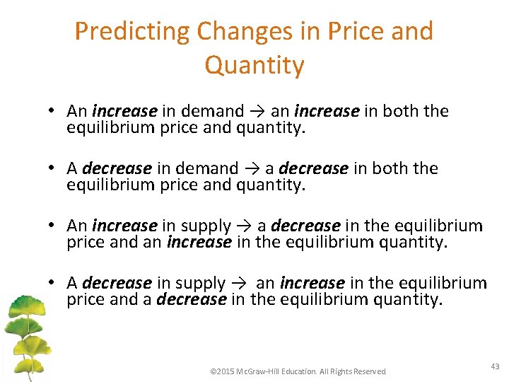
Predicting Changes in Price and Quantity • An increase in demand → an increase in both the equilibrium price and quantity. • A decrease in demand → a decrease in both the equilibrium price and quantity. • An increase in supply → a decrease in the equilibrium price and an increase in the equilibrium quantity. • A decrease in supply → an increase in the equilibrium price and a decrease in the equilibrium quantity. © 2015 Mc. Graw-Hill Education. All Rights Reserved. 43

PRICE CEILINGS – A price ceiling or price cap is a government regulation that places an upper limit on the price at which a particular good, service, or factor of production may be traded. – An example is a price ceiling on housing rents. – Trading above the price ceiling is illegal.

PRICE CEILINGS <A Rent Ceiling – A rent ceiling is a regulation that makes it illegal to charge more than a specified rent for housing. – The effect of a rent ceiling depends on whether it is imposed at a level above or below the market equilibrium rent.

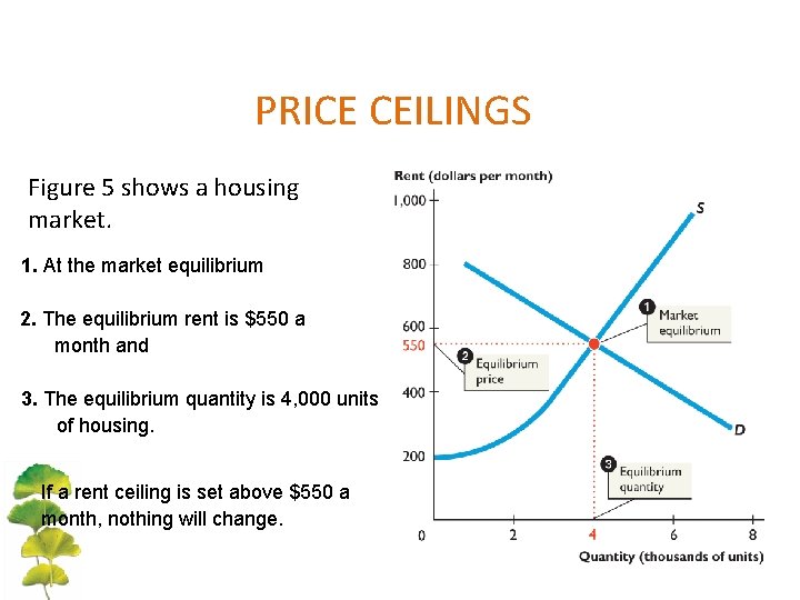
PRICE CEILINGS Figure 5 shows a housing market. 1. At the market equilibrium 2. The equilibrium rent is $550 a month and 3. The equilibrium quantity is 4, 000 units of housing. If a rent ceiling is set above $550 a month, nothing will change.

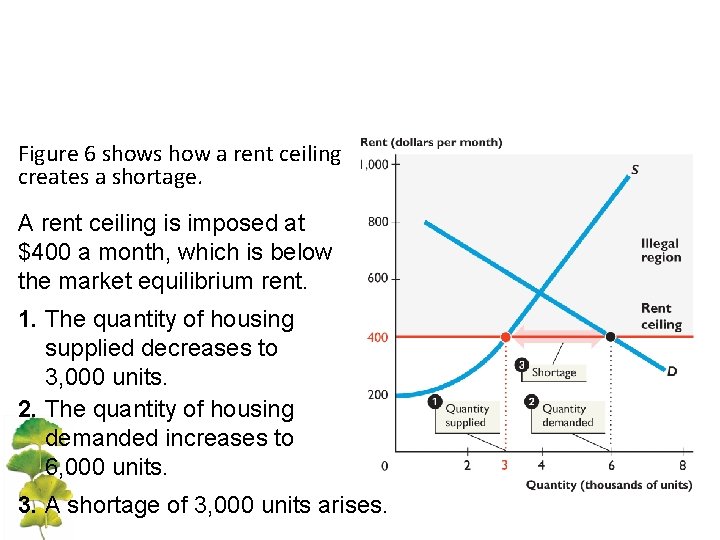
Figure 6 shows how a rent ceiling creates a shortage. A rent ceiling is imposed at $400 a month, which is below the market equilibrium rent. 1. The quantity of housing supplied decreases to 3, 000 units. 2. The quantity of housing demanded increases to 6, 000 units. 3. A shortage of 3, 000 units arises.

– When a rent ceiling creates a housing shortage, two developments occur: • A black market • Increased search activity – A black market is an illegal market that operates alongside a government-regulated market. – Search activity is the time spent looking for someone with whom to do business.

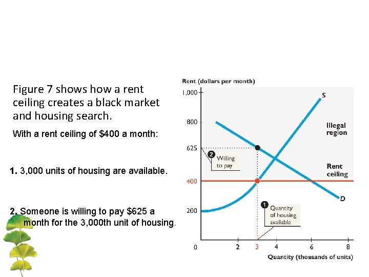
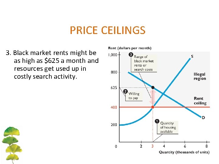
Figure 7 shows how a rent ceiling creates a black market and housing search. With a rent ceiling of $400 a month: 1. 3, 000 units of housing are available. 2. Someone is willing to pay $625 a month for the 3, 000 th unit of housing.

PRICE CEILINGS 3. Black market rents might be as high as $625 a month and resources get used up in costly search activity.

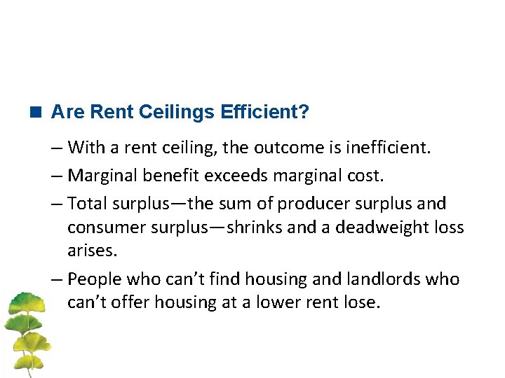
< Are Rent Ceilings Efficient? – With a rent ceiling, the outcome is inefficient. – Marginal benefit exceeds marginal cost. – Total surplus—the sum of producer surplus and consumer surplus—shrinks and a deadweight loss arises. – People who can’t find housing and landlords who can’t offer housing at a lower rent lose.

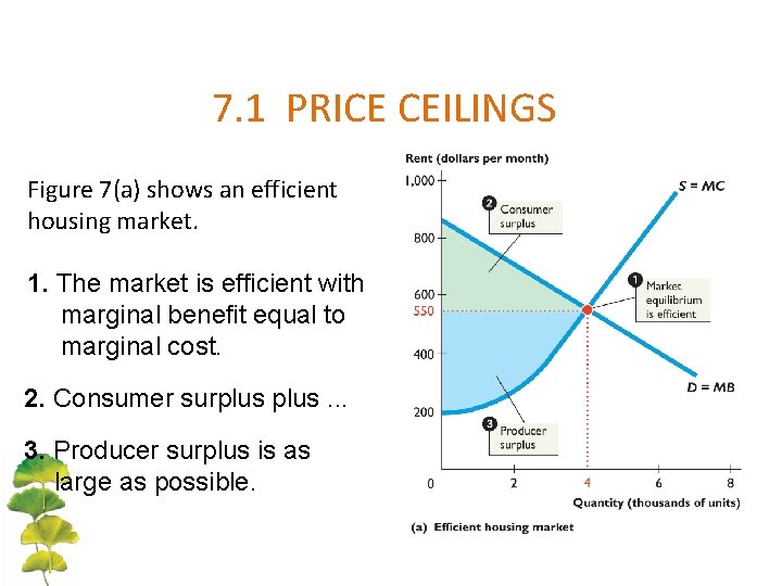
7. 1 PRICE CEILINGS Figure 7(a) shows an efficient housing market. 1. The market is efficient with marginal benefit equal to marginal cost. 2. Consumer surplus. . . 3. Producer surplus is as large as possible.

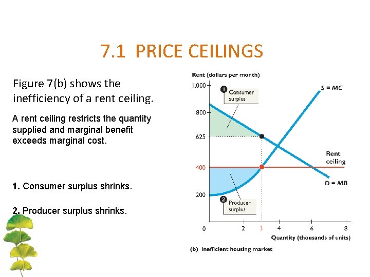
7. 1 PRICE CEILINGS Figure 7(b) shows the inefficiency of a rent ceiling. A rent ceiling restricts the quantity supplied and marginal benefit exceeds marginal cost. 1. Consumer surplus shrinks. 2. Producer surplus shrinks.

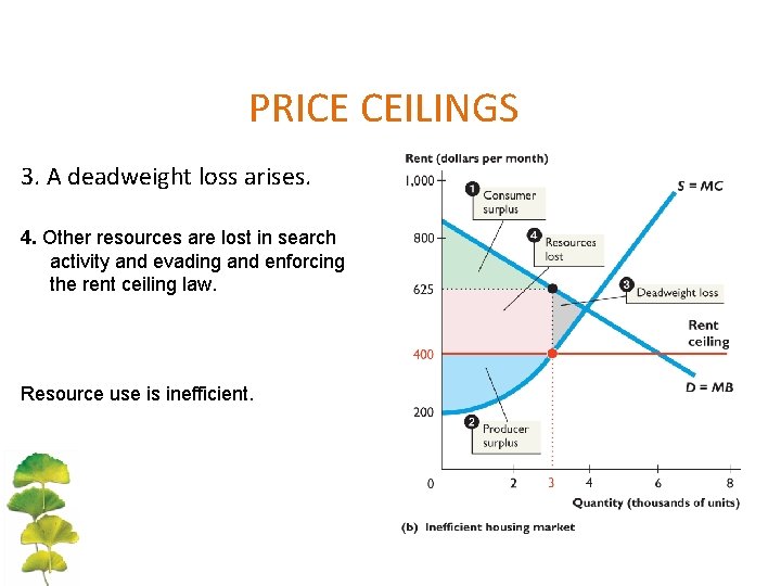
PRICE CEILINGS 3. A deadweight loss arises. 4. Other resources are lost in search activity and evading and enforcing the rent ceiling law. Resource use is inefficient.

PRICE FLOORS A price floor is a government regulation that places a lower limit on the price at which a particular good, service, or factor of production may be traded. – An example is the minimum wage in labor markets. – Trading below the price floor is illegal.

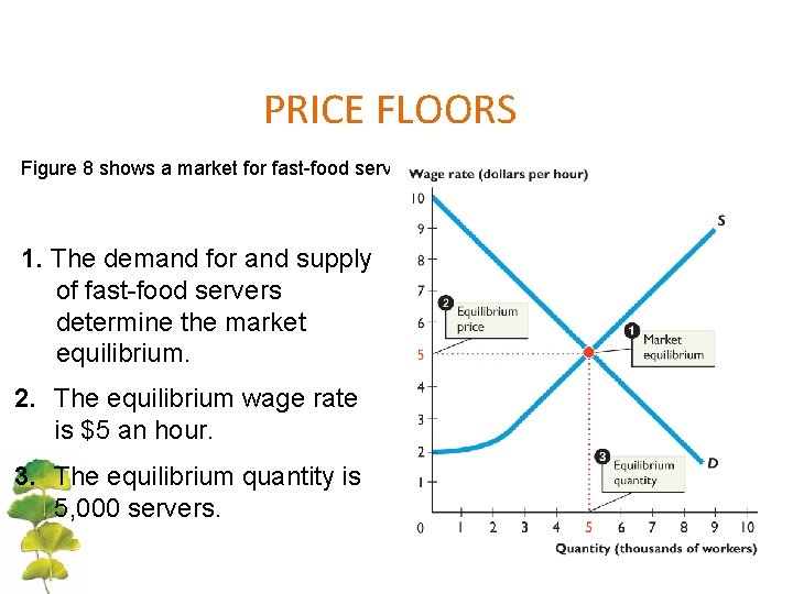
PRICE FLOORS Figure 8 shows a market for fast-food servers. 1. The demand for and supply of fast-food servers determine the market equilibrium. 2. The equilibrium wage rate is $5 an hour. 3. The equilibrium quantity is 5, 000 servers.

PRICE FLOORS <The Minimum Wage A minimum wage law is a government regulation that makes hiring labor for less than a specified wage illegal. –Firms can pay a wage rate above the minimum wage but they may not pay a wage rate below the minimum wage. –The effect of a minimum wage depends on whether it is set above or below the market equilibrium wage rate.

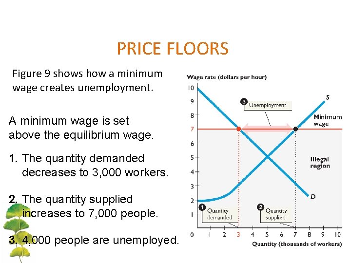
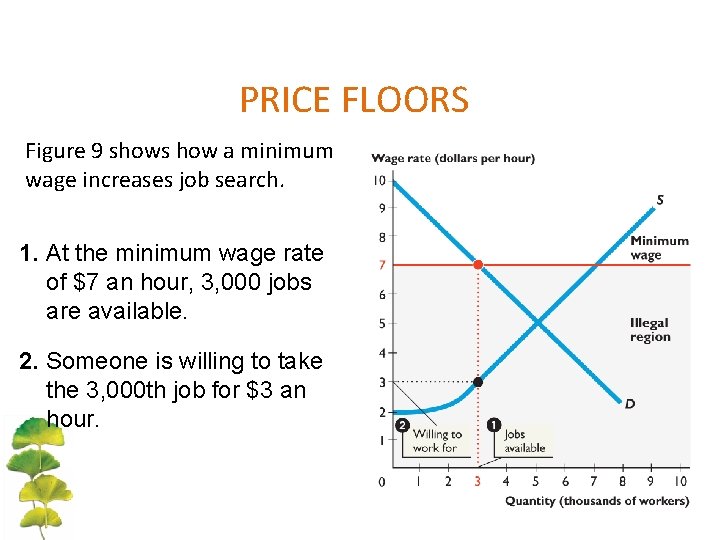
PRICE FLOORS Figure 9 shows how a minimum wage creates unemployment. A minimum wage is set above the equilibrium wage. 1. The quantity demanded decreases to 3, 000 workers. 2. The quantity supplied increases to 7, 000 people. 3. 4, 000 people are unemployed.

PRICE FLOORS –Of the 4, 000 people unemployed, 2, 000 have been fired another 2, 000 would like to work at $7 an hour. –The 3, 000 jobs must somehow be allocated to the 7, 000 people who would like to work. –This allocation is achieved by • Increased search activity • Illegal hiring

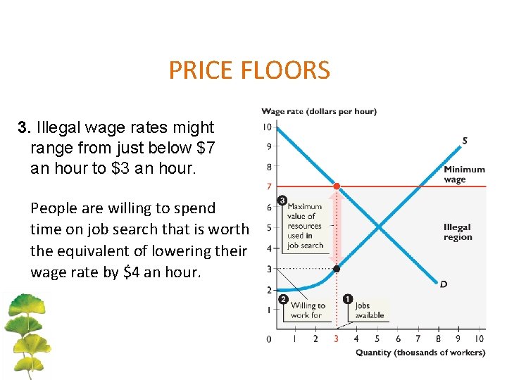
PRICE FLOORS Figure 9 shows how a minimum wage increases job search. 1. At the minimum wage rate of $7 an hour, 3, 000 jobs are available. 2. Someone is willing to take the 3, 000 th job for $3 an hour.

PRICE FLOORS 3. Illegal wage rates might range from just below $7 an hour to $3 an hour. People are willing to spend time on job search that is worth the equivalent of lowering their wage rate by $4 an hour.

<Is the Minimum Wage Efficient? – The firms’ surplus and workers’ surplus shrink, and a deadweight loss arises. – Firms that cut back employment and people who can’t find jobs at the higher wage rate lose. – The total loss exceeds the deadweight loss because resources get used in costly job-search activity.

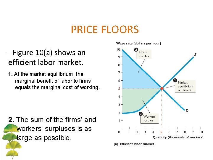
PRICE FLOORS – Figure 10(a) shows an efficient labor market. 1. At the market equilibrium, the marginal benefit of labor to firms equals the marginal cost of working. 2. The sum of the firms’ and workers’ surpluses is as large as possible.

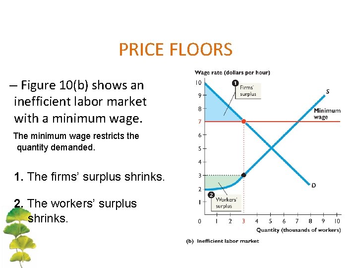
PRICE FLOORS – Figure 10(b) shows an inefficient labor market with a minimum wage. The minimum wage restricts the quantity demanded. 1. The firms’ surplus shrinks. 2. The workers’ surplus shrinks.

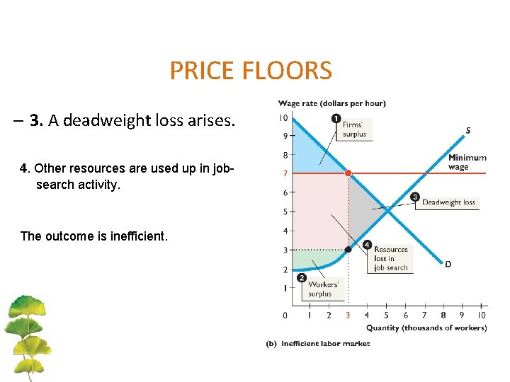
PRICE FLOORS – 3. A deadweight loss arises. 4. Other resources are used up in jobsearch activity. The outcome is inefficient.

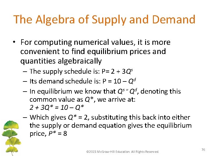
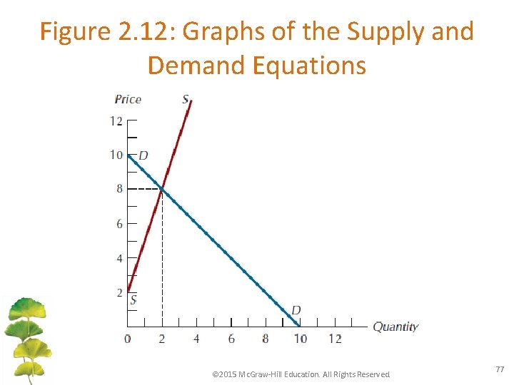
The Algebra of Supply and Demand • For computing numerical values, it is more convenient to find equilibrium prices and quantities algebraically – The supply schedule is: P= 2 + 3 Qs – Its demand schedule is: P = 10 – Qd – In equilibrium we know that Qs = Qd, denoting this common value as Q*, we arrive at: 2 + 3 Q* = 10 – Q* – Which gives Q* = 2, substituting this back into either the supply or demand equation gives the equilibrium price, P* = 8 © 2015 Mc. Graw-Hill Education. All Rights Reserved. 76

Figure 2. 12: Graphs of the Supply and Demand Equations © 2015 Mc. Graw-Hill Education. All Rights Reserved. 77

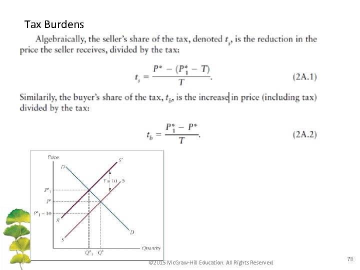
Tax Burdens © 2015 Mc. Graw-Hill Education. All Rights Reserved. 78

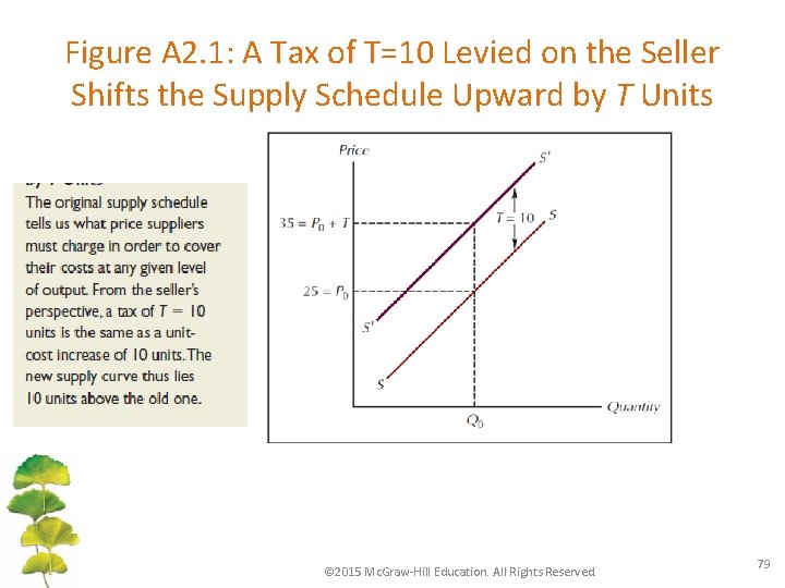
Figure A 2. 1: A Tax of T=10 Levied on the Seller Shifts the Supply Schedule Upward by T Units © 2015 Mc. Graw-Hill Education. All Rights Reserved. 79

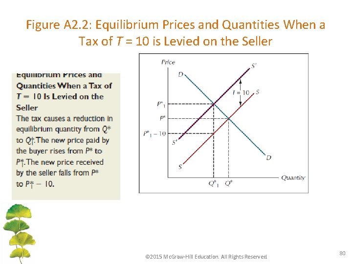
Figure A 2. 2: Equilibrium Prices and Quantities When a Tax of T = 10 is Levied on the Seller © 2015 Mc. Graw-Hill Education. All Rights Reserved. 80

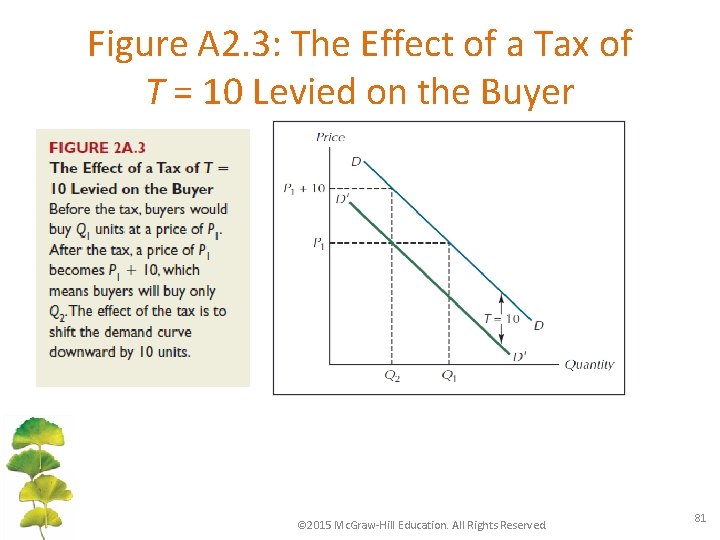
Figure A 2. 3: The Effect of a Tax of T = 10 Levied on the Buyer © 2015 Mc. Graw-Hill Education. All Rights Reserved. 81

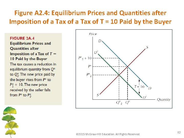
Figure A 2. 4: Equilibrium Prices and Quantities after Imposition of a Tax of T = 10 Paid by the Buyer © 2015 Mc. Graw-Hill Education. All Rights Reserved. 82

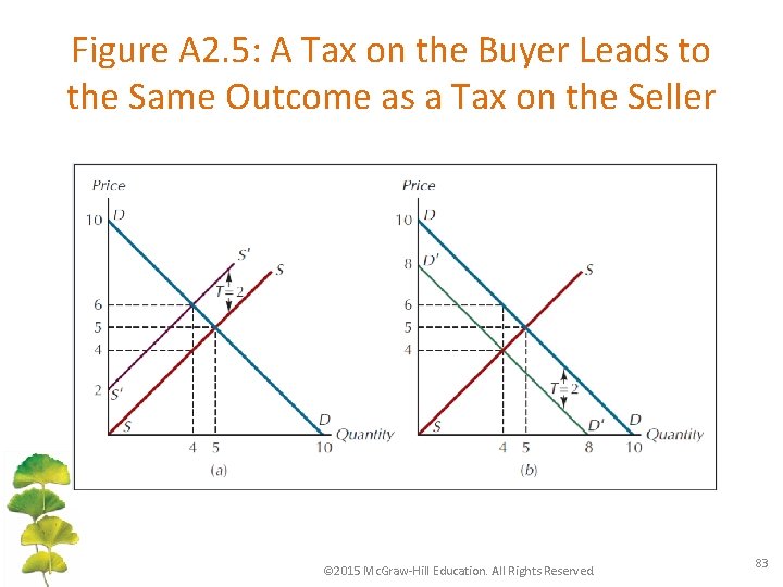
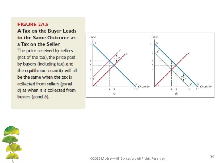
Figure A 2. 5: A Tax on the Buyer Leads to the Same Outcome as a Tax on the Seller © 2015 Mc. Graw-Hill Education. All Rights Reserved. 83

© 2015 Mc. Graw-Hill Education. All Rights Reserved. 84