Chapter 2 Simple Linear Regression RayBing Chen Institute

Chapter 2 Simple Linear Regression Ray-Bing Chen Institute of Statistics National University of Kaohsiung 1

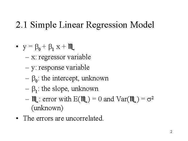
2. 1 Simple Linear Regression Model • y = 0 + 1 x + – x: regressor variable – y: response variable – 0: the intercept, unknown – 1: the slope, unknown – : error with E( ) = 0 and Var( ) = 2 (unknown) • The errors are uncorrelated. 2

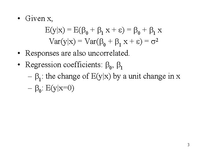
• Given x, E(y|x) = E( 0 + 1 x + ) = 0 + 1 x Var(y|x) = Var( 0 + 1 x + ) = 2 • Responses are also uncorrelated. • Regression coefficients: 0, 1 – 1: the change of E(y|x) by a unit change in x – 0: E(y|x=0) 3

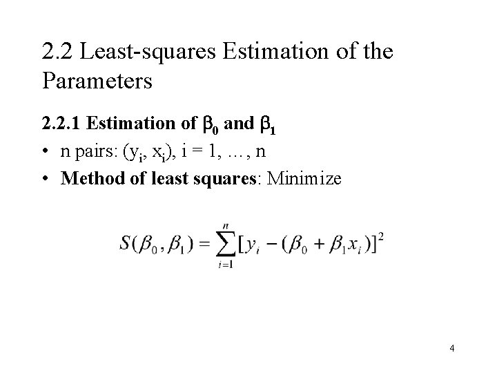
2. 2 Least-squares Estimation of the Parameters 2. 2. 1 Estimation of 0 and 1 • n pairs: (yi, xi), i = 1, …, n • Method of least squares: Minimize 4

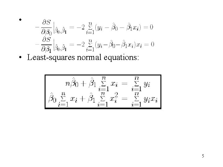
• • Least-squares normal equations: 5

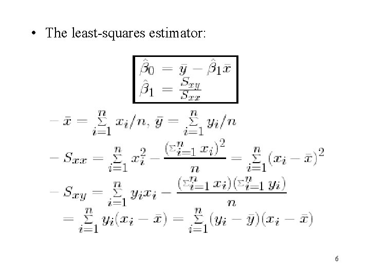
• The least-squares estimator: 6

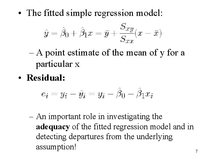
• The fitted simple regression model: – A point estimate of the mean of y for a particular x • Residual: – An important role in investigating the adequacy of the fitted regression model and in detecting departures from the underlying assumption! 7

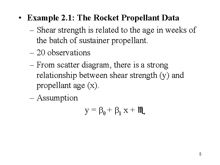
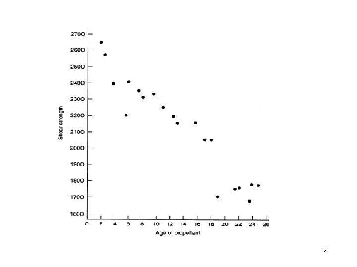
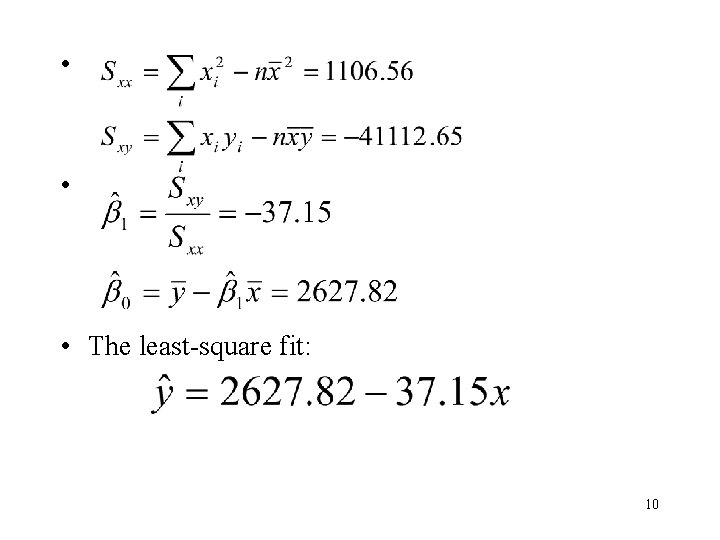
• Example 2. 1: The Rocket Propellant Data – Shear strength is related to the age in weeks of the batch of sustainer propellant. – 20 observations – From scatter diagram, there is a strong relationship between shear strength (y) and propellant age (x). – Assumption y = 0 + 1 x + 8

9

• • • The least-square fit: 10

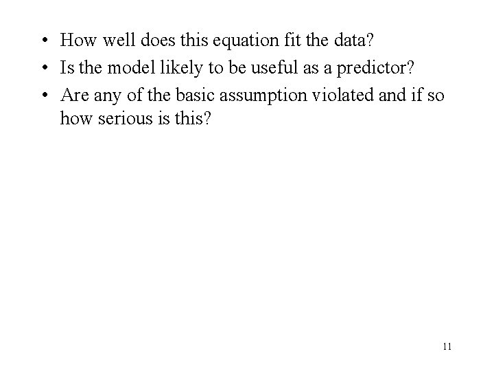
• How well does this equation fit the data? • Is the model likely to be useful as a predictor? • Are any of the basic assumption violated and if so how serious is this? 11

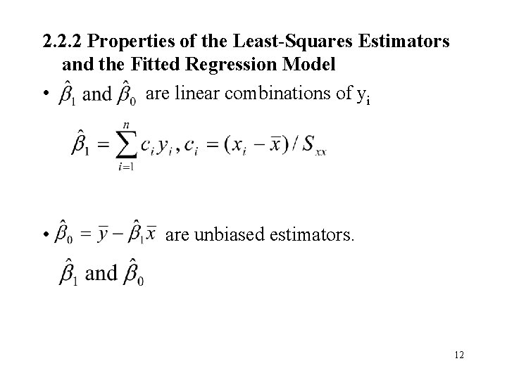
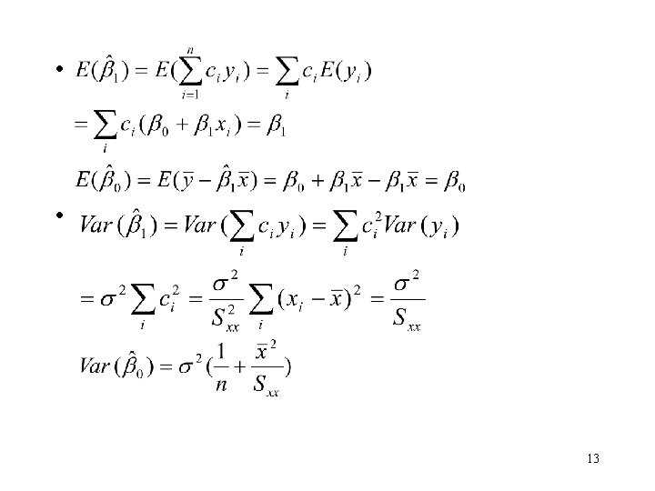
2. 2. 2 Properties of the Least-Squares Estimators and the Fitted Regression Model • are linear combinations of yi • are unbiased estimators. 12

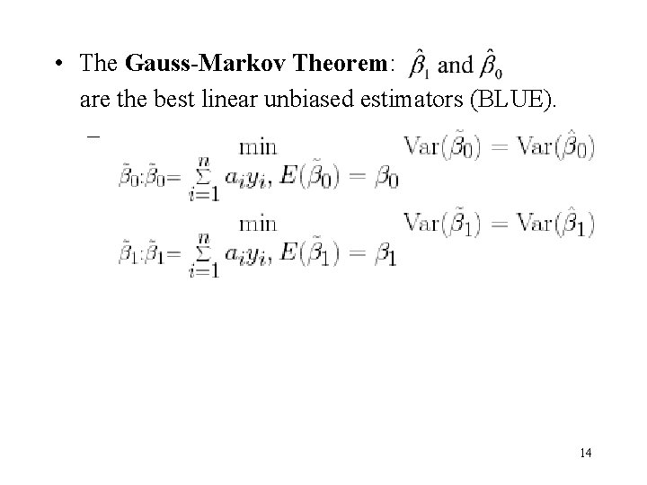
• The Gauss-Markov Theorem: are the best linear unbiased estimators (BLUE). – 14

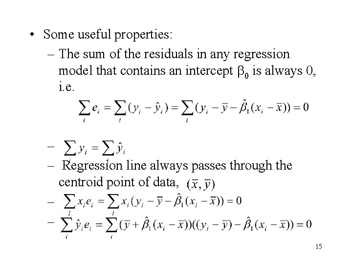
• Some useful properties: – The sum of the residuals in any regression model that contains an intercept 0 is always 0, i. e. – – Regression line always passes through the centroid point of data, – – 15

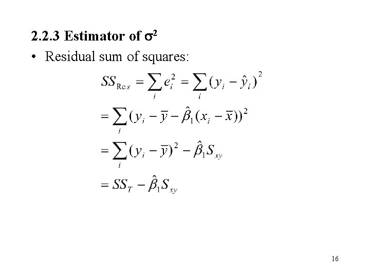
2. 2. 3 Estimator of 2 • Residual sum of squares: 16

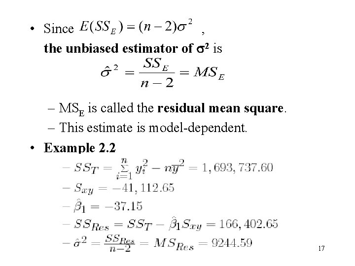
• Since , the unbiased estimator of 2 is – MSE is called the residual mean square. – This estimate is model-dependent. • Example 2. 2 17

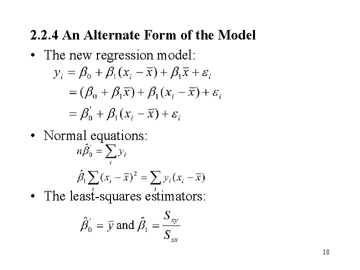
2. 2. 4 An Alternate Form of the Model • The new regression model: • Normal equations: • The least-squares estimators: 18

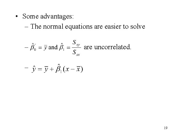
• Some advantages: – The normal equations are easier to solve – are uncorrelated. – 19

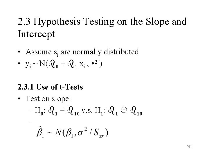
2. 3 Hypothesis Testing on the Slope and Intercept • Assume εi are normally distributed • yi ~ N( 0 + 1 xi , 2 ) 2. 3. 1 Use of t-Tests • Test on slope: – H 0: 1 = 10 v. s. H 1: 1 10 – 20

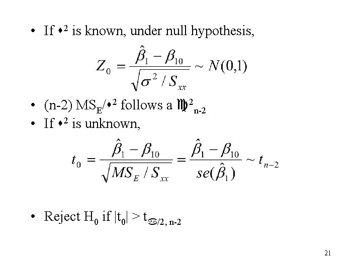
• If 2 is known, under null hypothesis, • (n-2) MSE/ 2 follows a 2 n-2 • If 2 is unknown, • Reject H 0 if |t 0| > t /2, n-2 21

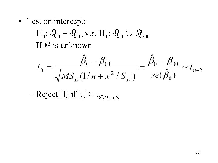
• Test on intercept: – H 0: 0 = 00 v. s. H 1: 0 00 – If 2 is unknown – Reject H 0 if |t 0| > t /2, n-2 22

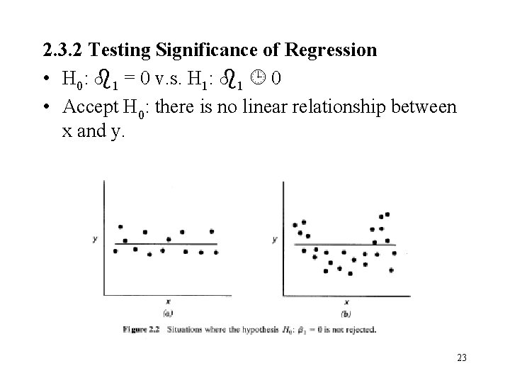
2. 3. 2 Testing Significance of Regression • H 0: 1 = 0 v. s. H 1: 1 0 • Accept H 0: there is no linear relationship between x and y. 23

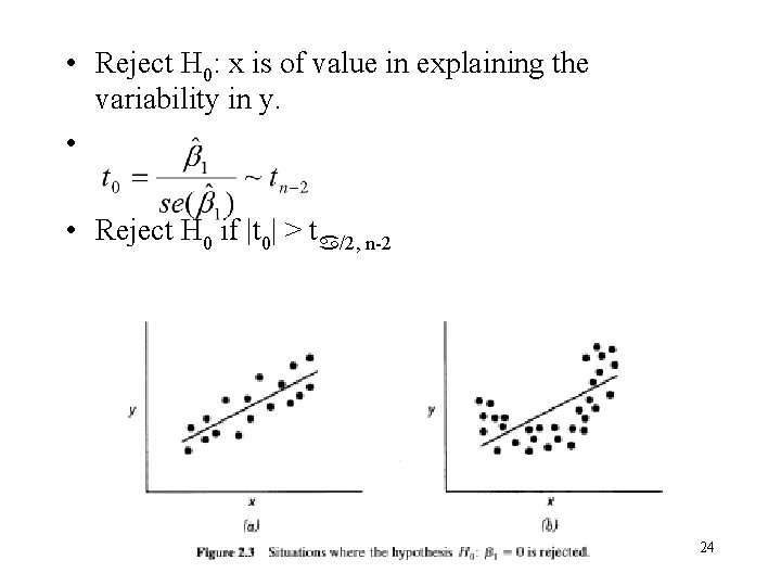
• Reject H 0: x is of value in explaining the variability in y. • • Reject H 0 if |t 0| > t /2, n-2 24

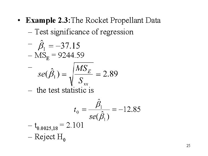
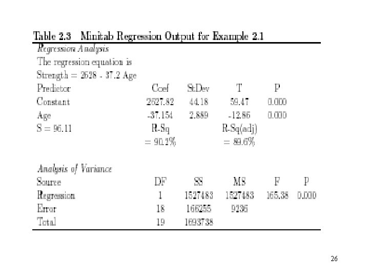
• Example 2. 3: The Rocket Propellant Data – Test significance of regression – – MSE = 9244. 59 – – the test statistic is – t 0. 0025, 18 = 2. 101 – Reject H 0 25

26

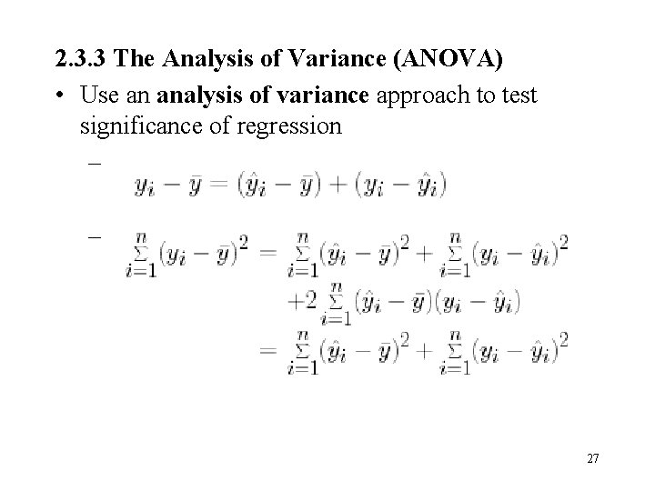
2. 3. 3 The Analysis of Variance (ANOVA) • Use an analysis of variance approach to test significance of regression – – 27

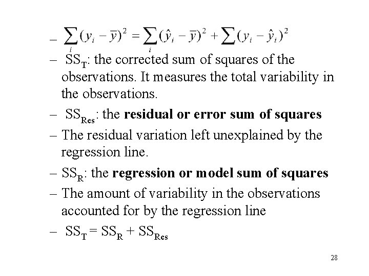
– – SST: the corrected sum of squares of the observations. It measures the total variability in the observations. – SSRes: the residual or error sum of squares – The residual variation left unexplained by the regression line. – SSR: the regression or model sum of squares – The amount of variability in the observations accounted for by the regression line – SST = SSR + SSRes 28

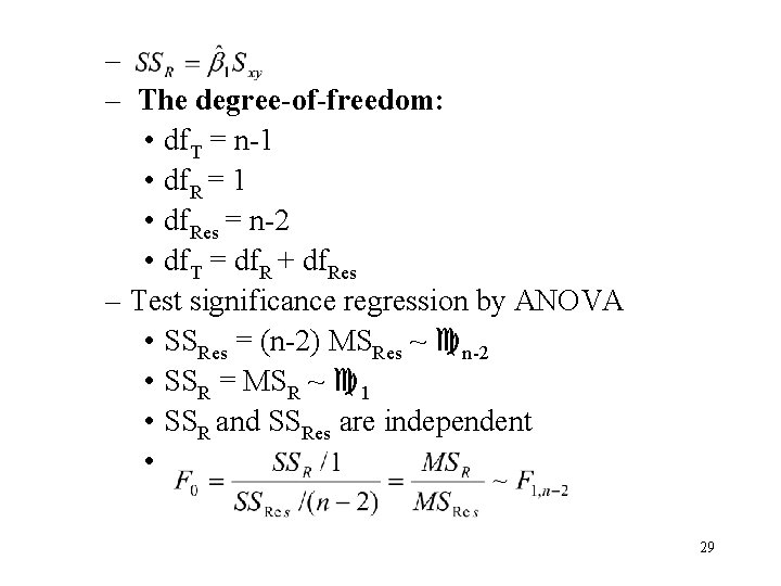
– – The degree-of-freedom: • df. T = n-1 • df. R = 1 • df. Res = n-2 • df. T = df. R + df. Res – Test significance regression by ANOVA • SSRes = (n-2) MSRes ~ n-2 • SSR = MSR ~ 1 • SSR and SSRes are independent • 29

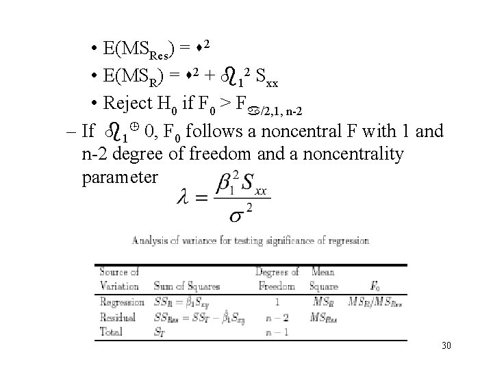
• E(MSRes) = 2 • E(MSR) = 2 + 12 Sxx • Reject H 0 if F 0 > F /2, 1, n-2 – If 1 0, F 0 follows a noncentral F with 1 and n-2 degree of freedom and a noncentrality parameter 30

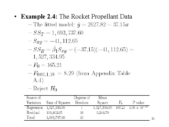
• Example 2. 4: The Rocket Propellant Data 31

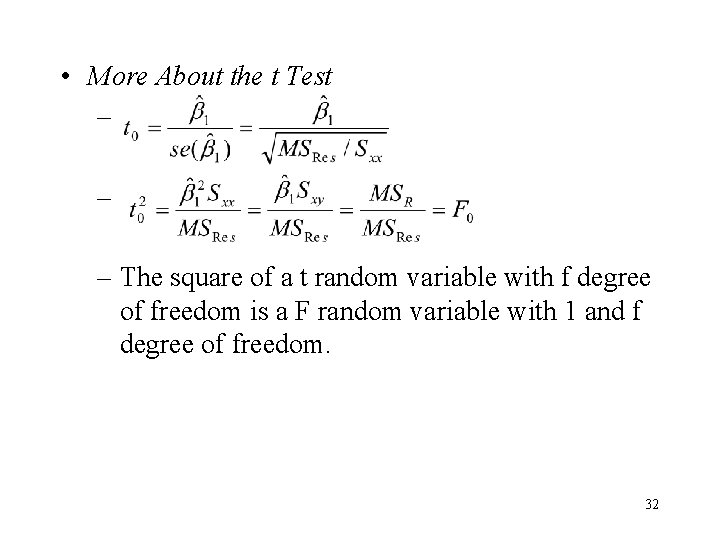
• More About the t Test – – – The square of a t random variable with f degree of freedom is a F random variable with 1 and f degree of freedom. 32

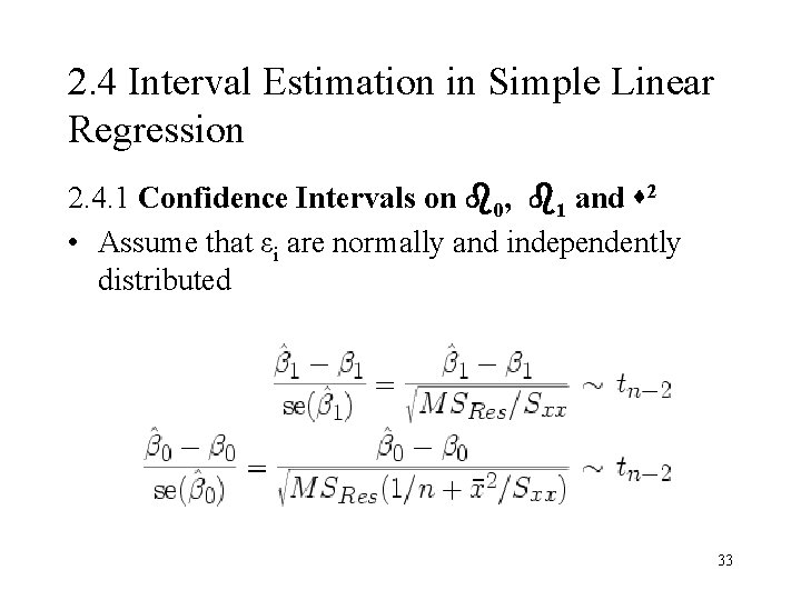
2. 4 Interval Estimation in Simple Linear Regression 2. 4. 1 Confidence Intervals on 0, 1 and 2 • Assume that εi are normally and independently distributed 33

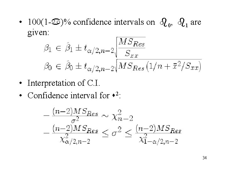
• 100(1 - )% confidence intervals on 0, 1 are given: • Interpretation of C. I. • Confidence interval for 2: 34

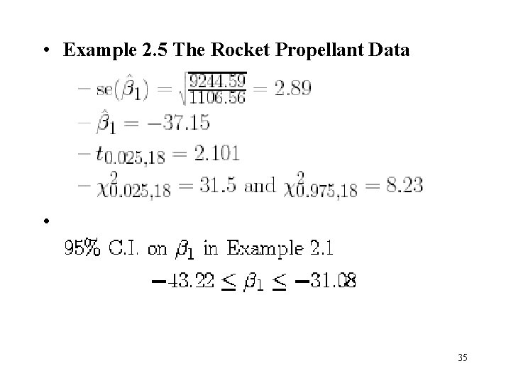
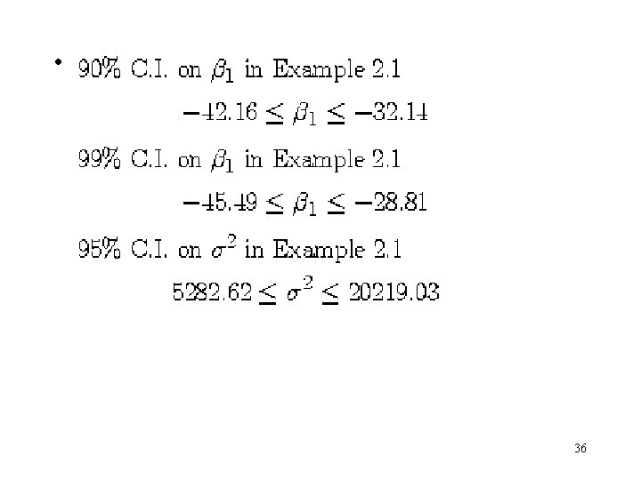
• Example 2. 5 The Rocket Propellant Data • 35

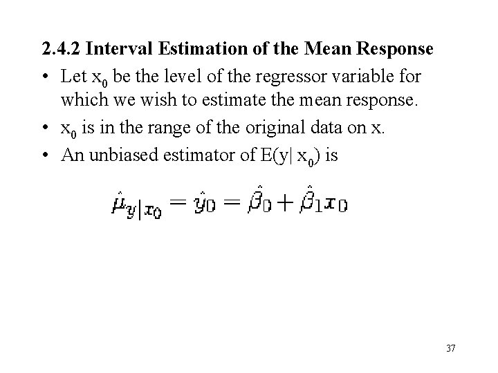
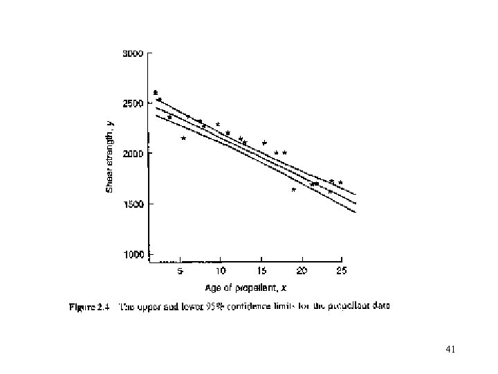
2. 4. 2 Interval Estimation of the Mean Response • Let x 0 be the level of the regressor variable for which we wish to estimate the mean response. • x 0 is in the range of the original data on x. • An unbiased estimator of E(y| x 0) is 37

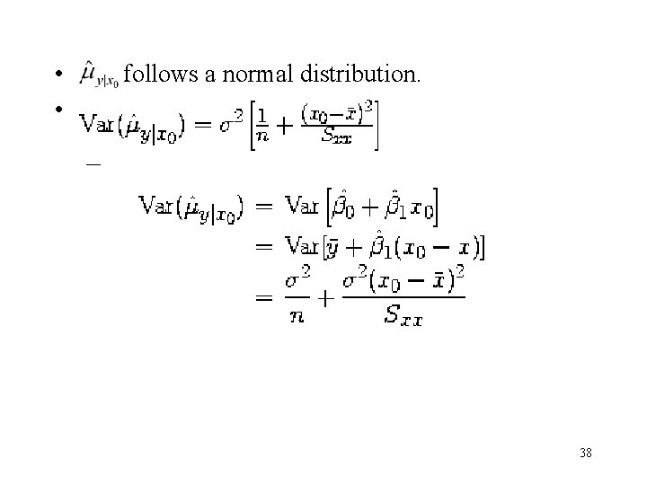
• • follows a normal distribution. 38

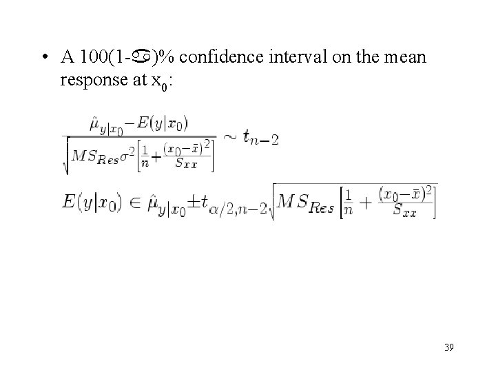
• A 100(1 - )% confidence interval on the mean response at x 0: 39

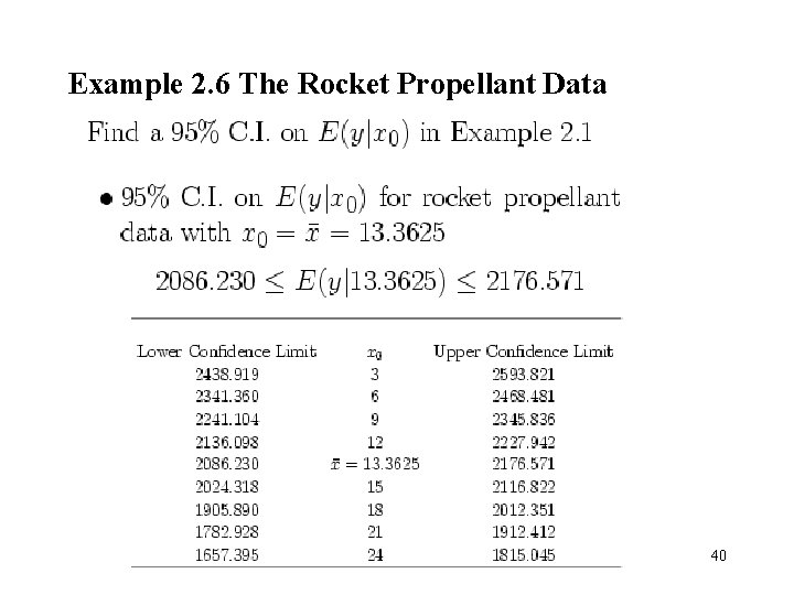
Example 2. 6 The Rocket Propellant Data 40

41

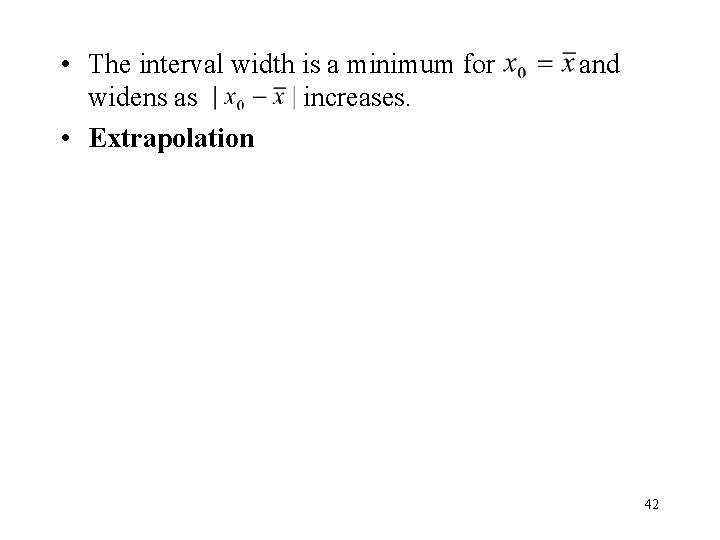
• The interval width is a minimum for widens as increases. • Extrapolation and 42

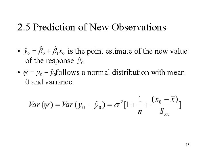
2. 5 Prediction of New Observations • is the point estimate of the new value of the response • follows a normal distribution with mean 0 and variance 43

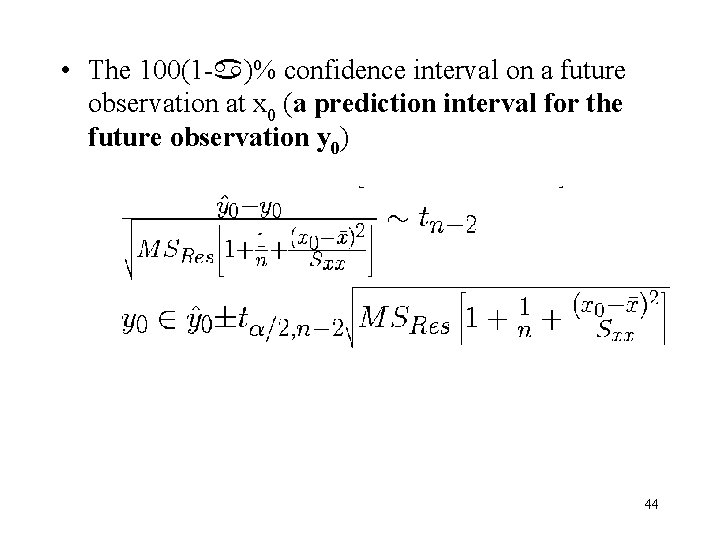
• The 100(1 - )% confidence interval on a future observation at x 0 (a prediction interval for the future observation y 0) 44

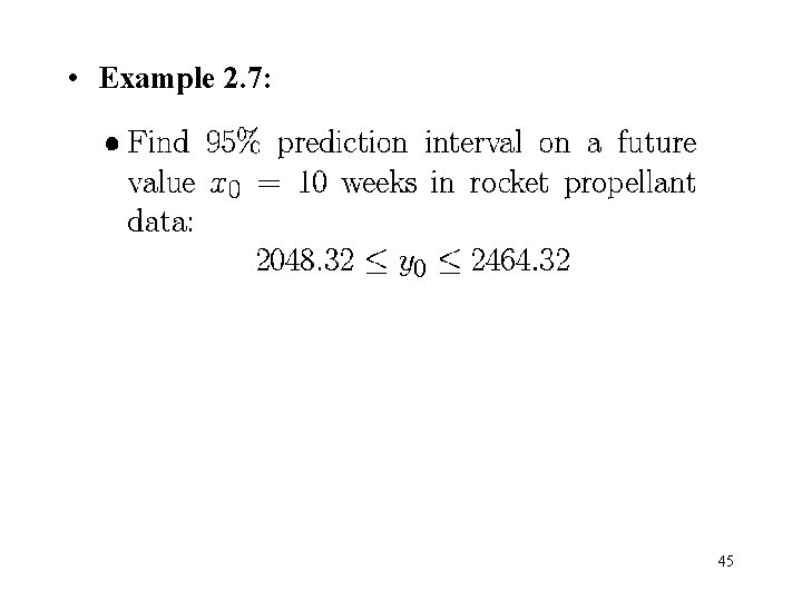
• Example 2. 7: 45

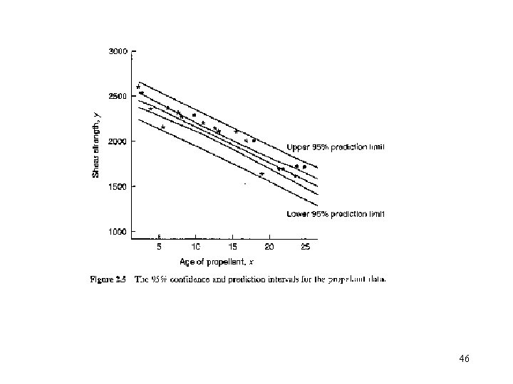
46

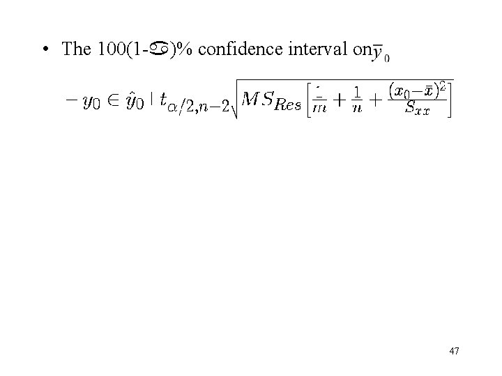
• The 100(1 - )% confidence interval on 47

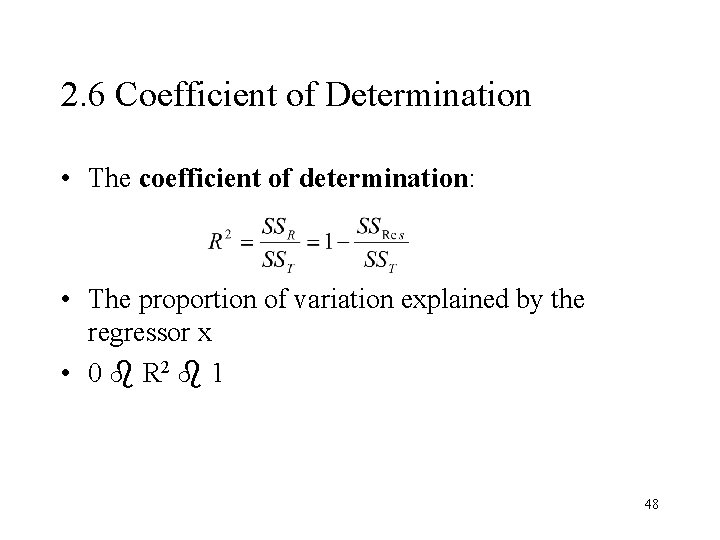
2. 6 Coefficient of Determination • The coefficient of determination: • The proportion of variation explained by the regressor x • 0 R 2 1 48

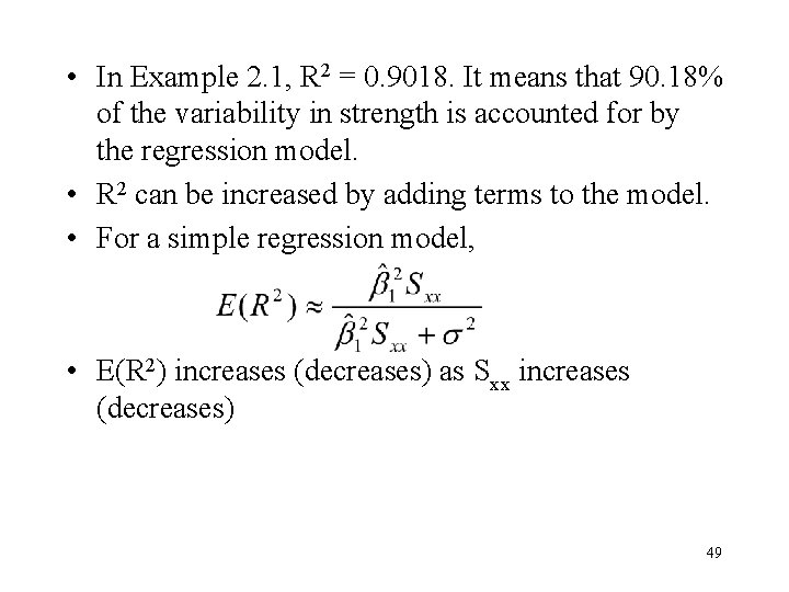
• In Example 2. 1, R 2 = 0. 9018. It means that 90. 18% of the variability in strength is accounted for by the regression model. • R 2 can be increased by adding terms to the model. • For a simple regression model, • E(R 2) increases (decreases) as Sxx increases (decreases) 49

• R 2 does not measure the magnitude of the slope of the regression line. A large value of R 2 imply a steep slope. • R 2 does not measure the appropriateness of the linear model. 50

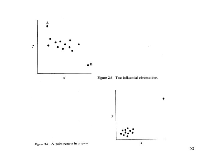
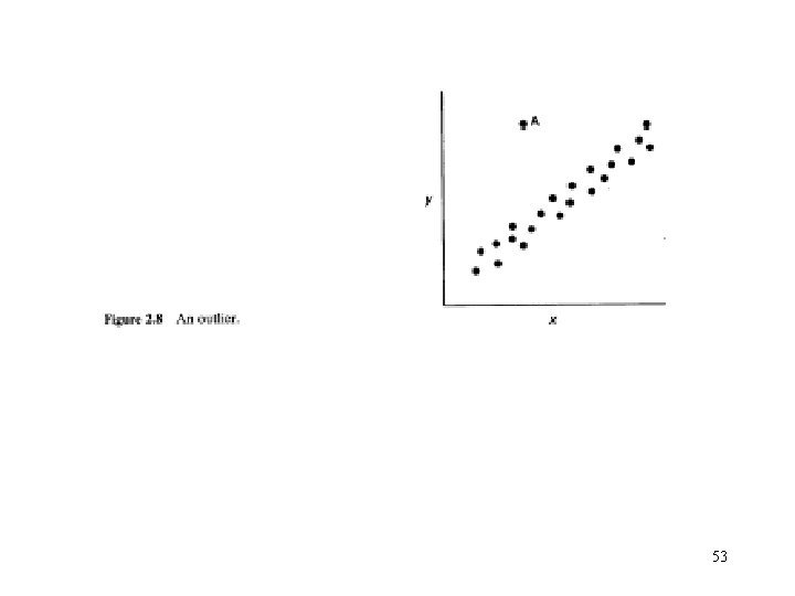
2. 7 Some Considerations in the Use of Regression • Only suitable for interpretation over the range of the regressors, not for extrapolation. • Important: The disposition of the x values. Slope strongly influenced by the remote values of x. • Outliers and bad values can seriously disturb the least-square fit. (intercept and the residual mean square) • Don’t imply the cause and effect relationship 51

52

53

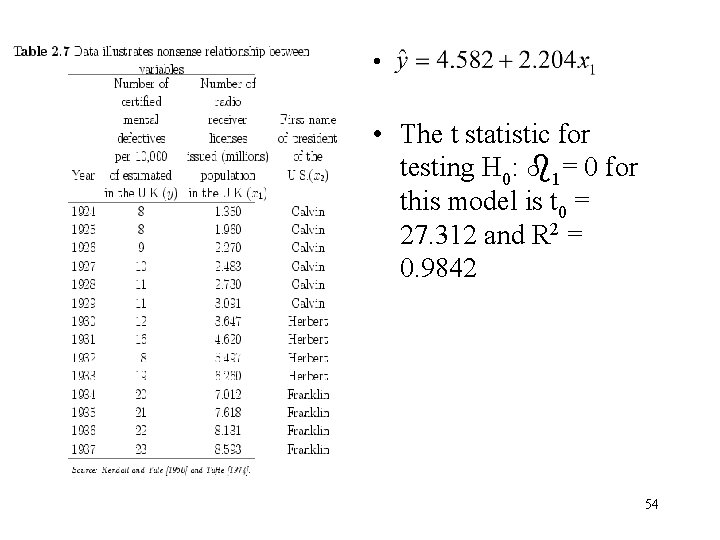
• • The t statistic for testing H 0: 1= 0 for this model is t 0 = 27. 312 and R 2 = 0. 9842 54

• x may be unknown. For example: consider predicting maximum daily load on an electric power generation system from a regression model relating the load to the maximum daily temperature. 55

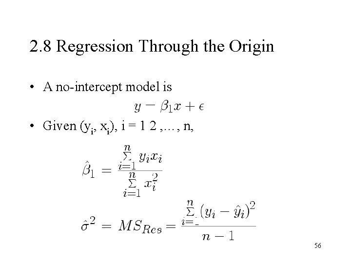
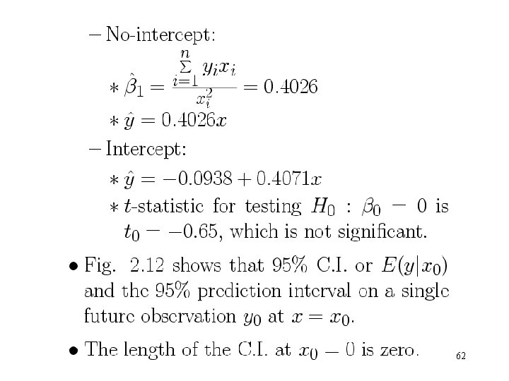
2. 8 Regression Through the Origin • A no-intercept model is • Given (yi, xi), i = 1 2 , …, n, 56

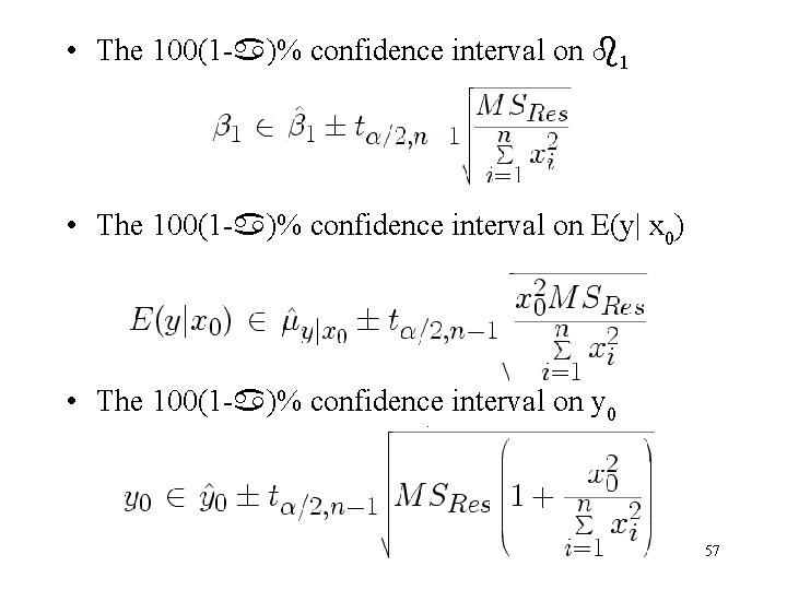
• The 100(1 - )% confidence interval on 1 • The 100(1 - )% confidence interval on E(y| x 0) • The 100(1 - )% confidence interval on y 0 57

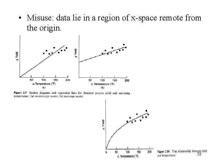
• Misuse: data lie in a region of x-space remote from the origin. 58

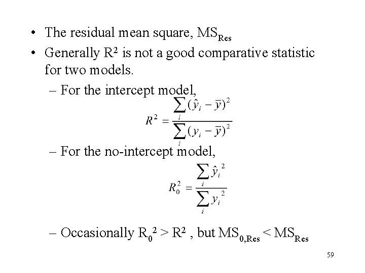
• The residual mean square, MSRes • Generally R 2 is not a good comparative statistic for two models. – For the intercept model, – For the no-intercept model, – Occasionally R 02 > R 2 , but MS 0, Res < MSRes 59

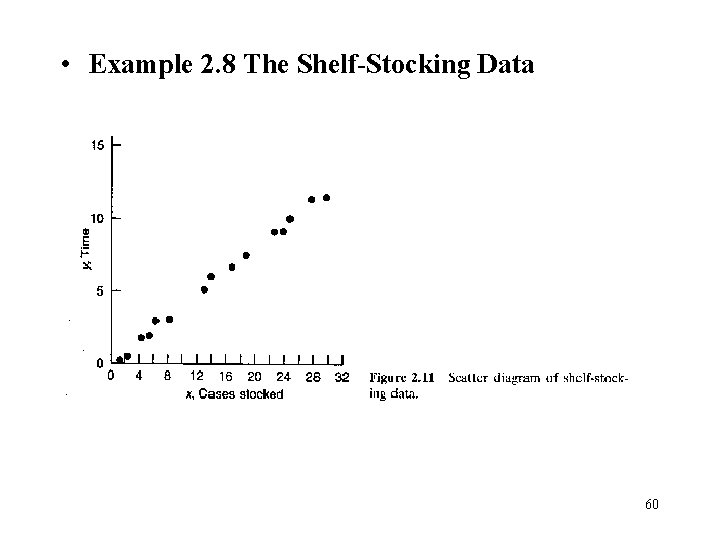
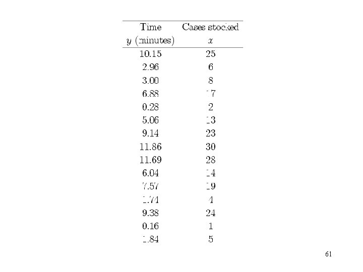
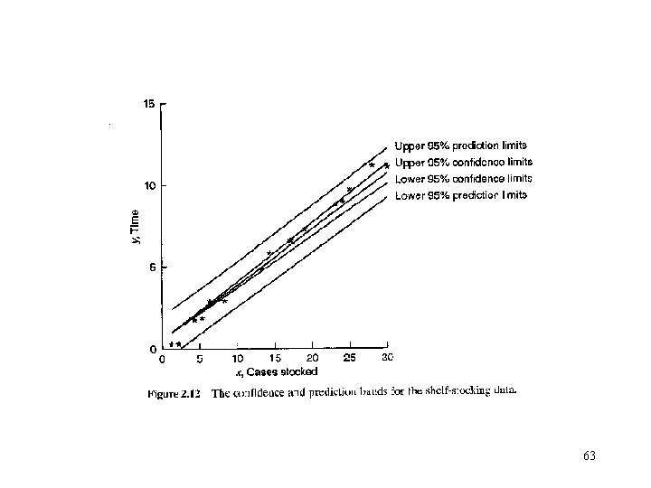
• Example 2. 8 The Shelf-Stocking Data 60

61

62

63

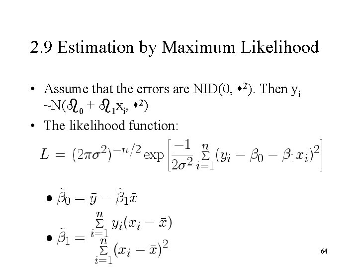
2. 9 Estimation by Maximum Likelihood • Assume that the errors are NID(0, 2). Then yi ~N( 0 + 1 xi, 2) • The likelihood function: 64

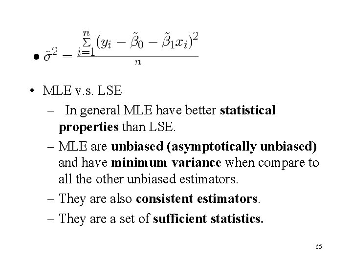
• MLE v. s. LSE – In general MLE have better statistical properties than LSE. – MLE are unbiased (asymptotically unbiased) and have minimum variance when compare to all the other unbiased estimators. – They are also consistent estimators. – They are a set of sufficient statistics. 65

– MLE requires more stringent statistical assumptions than LSE. – LSE only need to have the second moment assumptions. – MLE require a full distributional assumption. 66

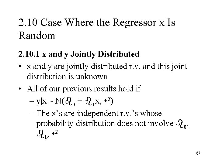
2. 10 Case Where the Regressor x Is Random 2. 10. 1 x and y Jointly Distributed • x and y are jointly distributed r. v. and this joint distribution is unknown. • All of our previous results hold if – y|x ~ N( 0 + 1 x, 2) – The x’s are independent r. v. ’s whose probability distribution does not involve 0, 1, 2 67

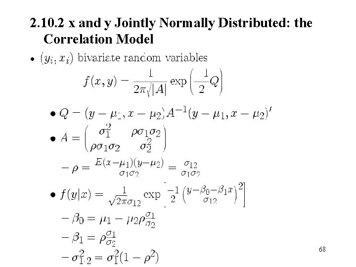
2. 10. 2 x and y Jointly Normally Distributed: the Correlation Model • 68

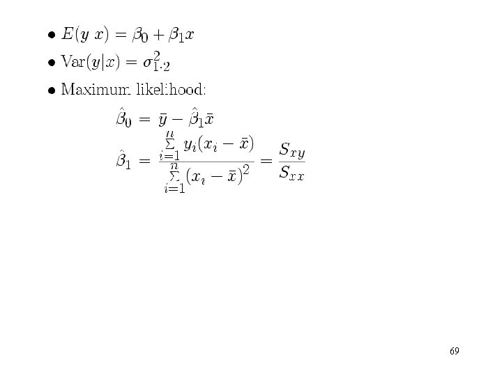
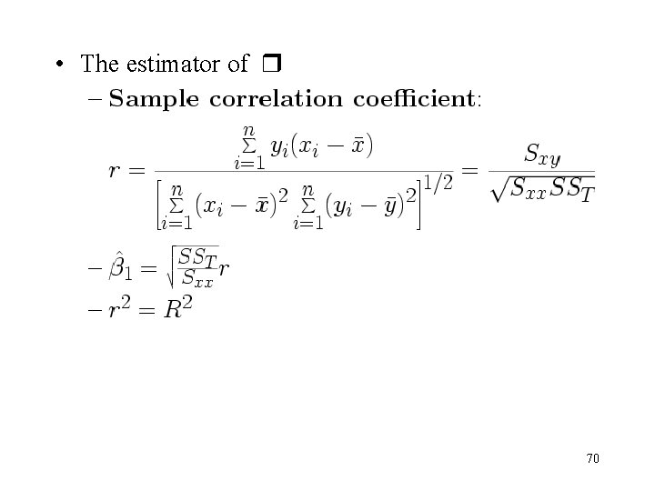
• The estimator of 70

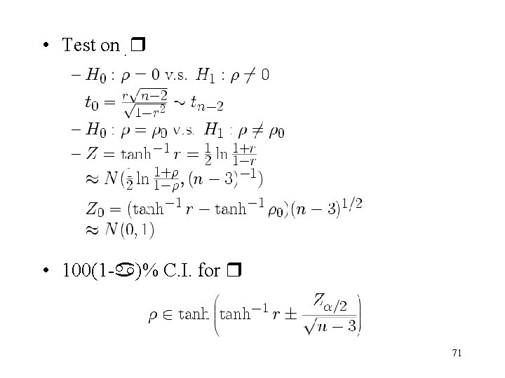
• Test on • 100(1 - )% C. I. for 71

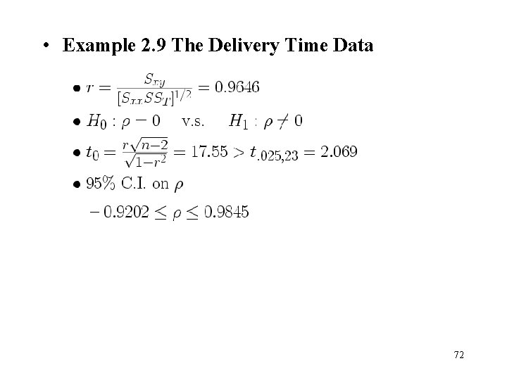
• Example 2. 9 The Delivery Time Data 72