Chapter 2 Section 2 Organizing Quantitative Data The

Chapter 2 Section 2 Organizing Quantitative Data: The Popular Displays Sullivan – Statistics: Informed Decisions Using Data – 2 nd Edition – Chapter 2 Section 2 – Slide 1 of 34

Chapter 2 – Section 2 ● Learning objectives 1 § 2 § 3 § 4 § 5 § 6 § 7 § Organize discrete data in tables Construct histograms of discrete data Organize continuous data in tables Construct histograms of continuous data Draw stem-and-leaf plots Draw dot plots Identify the shape of a distribution Sullivan – Statistics: Informed Decisions Using Data – 2 nd Edition – Chapter 2 Section 2 – Slide 2 of 34

Chapter 2 – Section 2 ● Learning objectives 1 § 2 § 3 § 4 § 5 § 6 § 7 § Organize discrete data in tables Construct histograms of discrete data Organize continuous data in tables Construct histograms of continuous data Draw stem-and-leaf plots Draw dot plots Identify the shape of a distribution Sullivan – Statistics: Informed Decisions Using Data – 2 nd Edition – Chapter 2 Section 2 – Slide 3 of 34

Chapter 2 – Section 2 ● Raw quantitative data comes as a list of values … each value is a measurement, either discrete or continuous ● Comparisons (one value being more than or less than another) can be performed on the data values ● Mathematical operations (addition, subtraction, …) can be performed on the data values Sullivan – Statistics: Informed Decisions Using Data – 2 nd Edition – Chapter 2 Section 2 – Slide 4 of 34

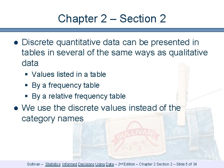
Chapter 2 – Section 2 ● Discrete quantitative data can be presented in tables in several of the same ways as qualitative data § Values listed in a table § By a frequency table § By a relative frequency table ● We use the discrete values instead of the category names Sullivan – Statistics: Informed Decisions Using Data – 2 nd Edition – Chapter 2 Section 2 – Slide 5 of 34

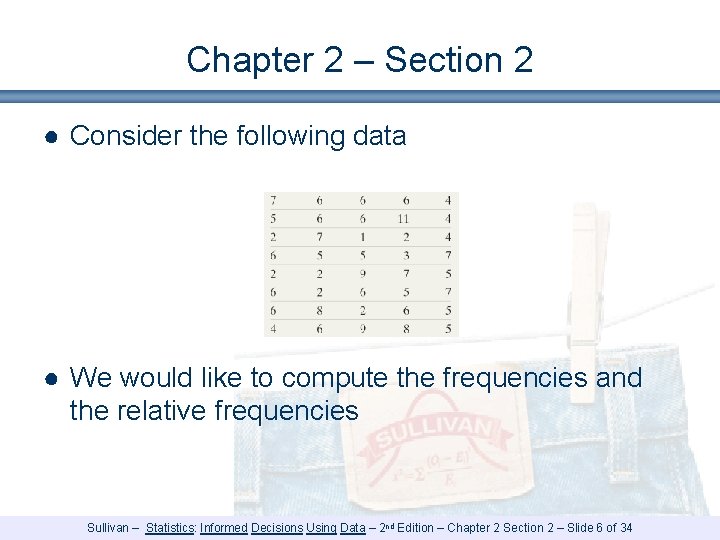
Chapter 2 – Section 2 ● Consider the following data ● We would like to compute the frequencies and the relative frequencies Sullivan – Statistics: Informed Decisions Using Data – 2 nd Edition – Chapter 2 Section 2 – Slide 6 of 34

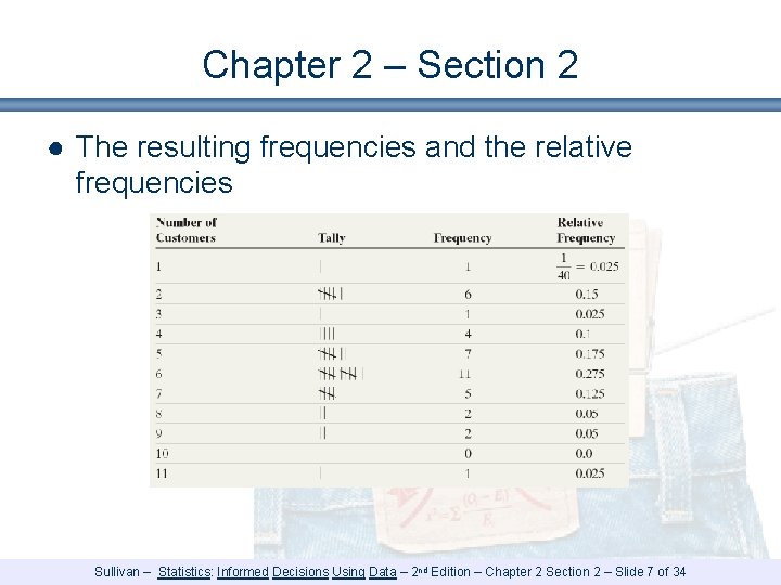
Chapter 2 – Section 2 ● The resulting frequencies and the relative frequencies Sullivan – Statistics: Informed Decisions Using Data – 2 nd Edition – Chapter 2 Section 2 – Slide 7 of 34

Chapter 2 – Section 2 ● Learning objectives 1 § 2 § 3 § 4 § 5 § 6 § 7 § Organize discrete data in tables Construct histograms of discrete data Organize continuous data in tables Construct histograms of continuous data Draw stem-and-leaf plots Draw dot plots Identify the shape of a distribution Sullivan – Statistics: Informed Decisions Using Data – 2 nd Edition – Chapter 2 Section 2 – Slide 8 of 34

Chapter 2 – Section 2 ● Discrete quantitative data can be presented in bar graphs in several of the same ways as qualitative data ● We use the discrete values instead of the category names ● We arrange the values in ascending order ● For discrete data, these are called histograms Sullivan – Statistics: Informed Decisions Using Data – 2 nd Edition – Chapter 2 Section 2 – Slide 9 of 34

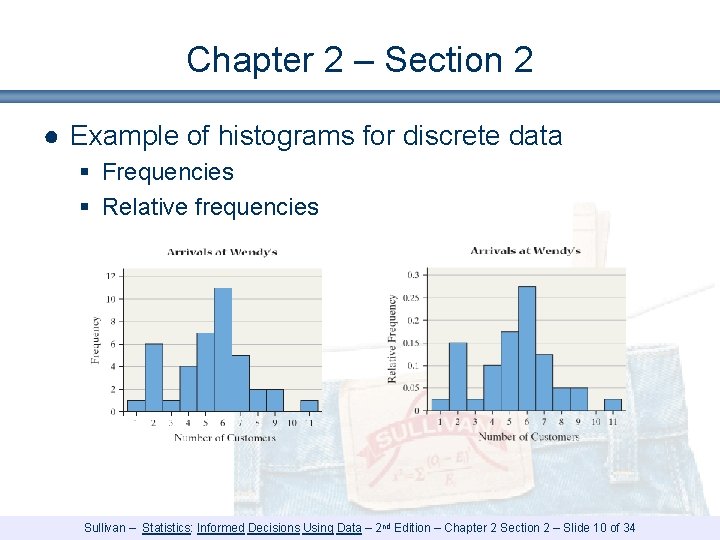
Chapter 2 – Section 2 ● Example of histograms for discrete data § Frequencies § Relative frequencies Sullivan – Statistics: Informed Decisions Using Data – 2 nd Edition – Chapter 2 Section 2 – Slide 10 of 34

Chapter 2 – Section 2 ● Learning objectives 1 § 2 § 3 § 4 § 5 § 6 § 7 § Organize discrete data in tables Construct histograms of discrete data Organize continuous data in tables Construct histograms of continuous data Draw stem-and-leaf plots Draw dot plots Identify the shape of a distribution Sullivan – Statistics: Informed Decisions Using Data – 2 nd Edition – Chapter 2 Section 2 – Slide 11 of 34

Chapter 2 – Section 2 ● Continuous data cannot be put directly into frequency tables since they do not have any obvious categories ● Categories are created using classes, or intervals of numbers ● The continuous data is then put into the classes Sullivan – Statistics: Informed Decisions Using Data – 2 nd Edition – Chapter 2 Section 2 – Slide 12 of 34

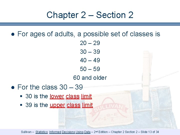
Chapter 2 – Section 2 ● For ages of adults, a possible set of classes is 20 – 29 30 – 39 40 – 49 50 – 59 60 and older ● For the class 30 – 39 § 30 is the lower class limit § 39 is the upper class limit Sullivan – Statistics: Informed Decisions Using Data – 2 nd Edition – Chapter 2 Section 2 – Slide 13 of 34

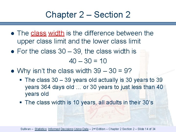
Chapter 2 – Section 2 ● The class width is the difference between the upper class limit and the lower class limit ● For the class 30 – 39, the class width is 40 – 30 = 10 ● Why isn’t the class width 39 – 30 = 9? § The class 30 – 39 years old actually is 30 years to 39 years 364 days old … or 30 years to just less than 40 years old § The class width is 10 years, all adults in their 30’s Sullivan – Statistics: Informed Decisions Using Data – 2 nd Edition – Chapter 2 Section 2 – Slide 14 of 34

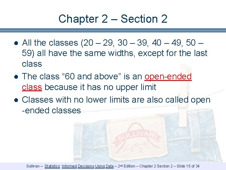
Chapter 2 – Section 2 ● All the classes (20 – 29, 30 – 39, 40 – 49, 50 – 59) all have the same widths, except for the last class ● The class “ 60 and above” is an open-ended class because it has no upper limit ● Classes with no lower limits are also called open -ended classes Sullivan – Statistics: Informed Decisions Using Data – 2 nd Edition – Chapter 2 Section 2 – Slide 15 of 34

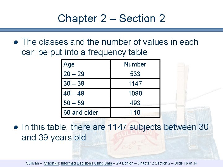
Chapter 2 – Section 2 ● The classes and the number of values in each can be put into a frequency table Age Number 20 – 29 533 30 – 39 1147 40 – 49 1090 50 – 59 493 60 and older 110 ● In this table, there are 1147 subjects between 30 and 39 years old Sullivan – Statistics: Informed Decisions Using Data – 2 nd Edition – Chapter 2 Section 2 – Slide 16 of 34

Chapter 2 – Section 2 ● Good practices for constructing tables for continuous variables § The classes should not overlap § The classes should not have any gaps between them § The classes should have the same width (except for possible open-ended classes at the extreme low or extreme high ends) § The class boundaries should be “reasonable” numbers § The class width should be a “reasonable” number Sullivan – Statistics: Informed Decisions Using Data – 2 nd Edition – Chapter 2 Section 2 – Slide 17 of 34

Chapter 2 – Section 2 ● Learning objectives 1 § 2 § 3 § 4 § 5 § 6 § 7 § Organize discrete data in tables Construct histograms of discrete data Organize continuous data in tables Construct histograms of continuous data Draw stem-and-leaf plots Draw dot plots Identify the shape of a distribution Sullivan – Statistics: Informed Decisions Using Data – 2 nd Edition – Chapter 2 Section 2 – Slide 18 of 34

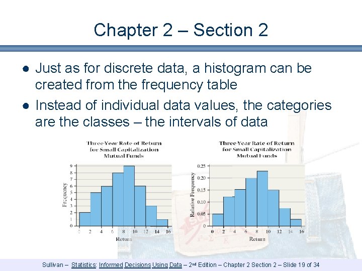
Chapter 2 – Section 2 ● Just as for discrete data, a histogram can be created from the frequency table ● Instead of individual data values, the categories are the classes – the intervals of data Sullivan – Statistics: Informed Decisions Using Data – 2 nd Edition – Chapter 2 Section 2 – Slide 19 of 34

Chapter 2 – Section 2 ● Learning objectives 1 § 2 § 3 § 4 § 5 § 6 § 7 § Organize discrete data in tables Construct histograms of discrete data Organize continuous data in tables Construct histograms of continuous data Draw stem-and-leaf plots Draw dot plots Identify the shape of a distribution Sullivan – Statistics: Informed Decisions Using Data – 2 nd Edition – Chapter 2 Section 2 – Slide 20 of 34

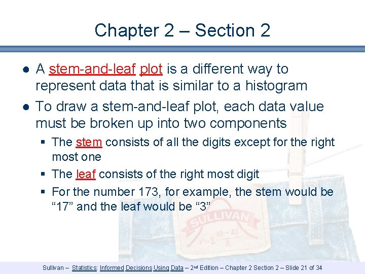
Chapter 2 – Section 2 ● A stem-and-leaf plot is a different way to represent data that is similar to a histogram ● To draw a stem-and-leaf plot, each data value must be broken up into two components § The stem consists of all the digits except for the right most one § The leaf consists of the right most digit § For the number 173, for example, the stem would be “ 17” and the leaf would be “ 3” Sullivan – Statistics: Informed Decisions Using Data – 2 nd Edition – Chapter 2 Section 2 – Slide 21 of 34

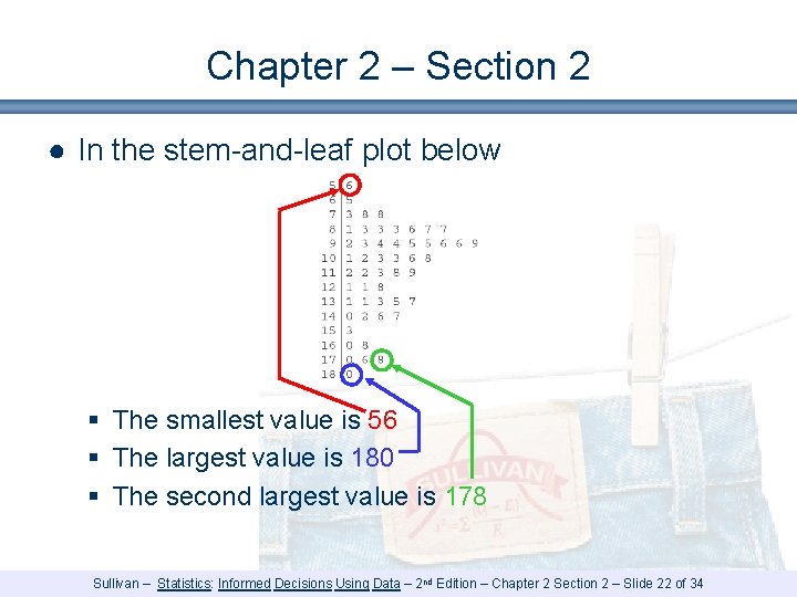
Chapter 2 – Section 2 ● In the stem-and-leaf plot below § The smallest value is 56 § The largest value is 180 § The second largest value is 178 Sullivan – Statistics: Informed Decisions Using Data – 2 nd Edition – Chapter 2 Section 2 – Slide 22 of 34

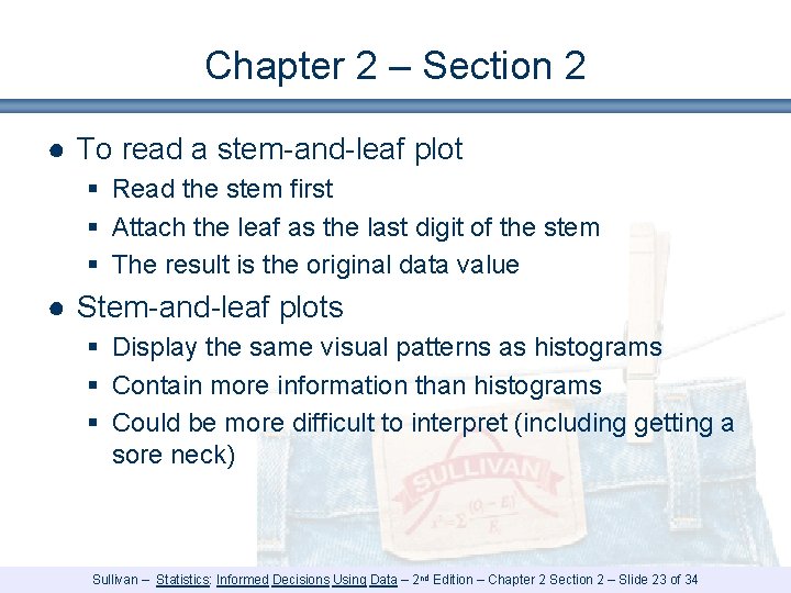
Chapter 2 – Section 2 ● To read a stem-and-leaf plot § Read the stem first § Attach the leaf as the last digit of the stem § The result is the original data value ● Stem-and-leaf plots § Display the same visual patterns as histograms § Contain more information than histograms § Could be more difficult to interpret (including getting a sore neck) Sullivan – Statistics: Informed Decisions Using Data – 2 nd Edition – Chapter 2 Section 2 – Slide 23 of 34

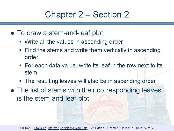
Chapter 2 – Section 2 ● To draw a stem-and-leaf plot § Write all the values in ascending order § Find the stems and write them vertically in ascending order § For each data value, write its leaf in the row next to its stem § The resulting leaves will also be in ascending order ● The list of stems with their corresponding leaves is the stem-and-leaf plot Sullivan – Statistics: Informed Decisions Using Data – 2 nd Edition – Chapter 2 Section 2 – Slide 24 of 34

Chapter 2 – Section 2 ● Modifications to stem-and-leaf plots § Sometimes there are too many values with the same stem … we would need to split the stems (such as having 10 -14 in one stem and 15 -19 in another) § If we wanted to compare two sets of data, we could draw two stem-and-leaf plots using the same stem, with leaves going left (for one set of data) and right (for the other set) § There are cases where constructing a descending stem-and-leaf plot could also be appropriate (for test scores, for example) Sullivan – Statistics: Informed Decisions Using Data – 2 nd Edition – Chapter 2 Section 2 – Slide 25 of 34

Chapter 2 – Section 2 ● Learning objectives 1 § 2 § 3 § 4 § 5 § 6 § 7 § Organize discrete data in tables Construct histograms of discrete data Organize continuous data in tables Construct histograms of continuous data Draw stem-and-leaf plots Draw dot plots Identify the shape of a distribution Sullivan – Statistics: Informed Decisions Using Data – 2 nd Edition – Chapter 2 Section 2 – Slide 26 of 34

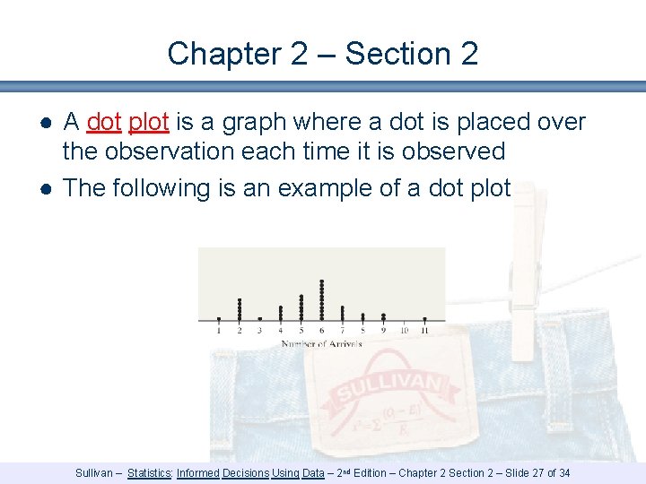
Chapter 2 – Section 2 ● A dot plot is a graph where a dot is placed over the observation each time it is observed ● The following is an example of a dot plot Sullivan – Statistics: Informed Decisions Using Data – 2 nd Edition – Chapter 2 Section 2 – Slide 27 of 34

Chapter 2 – Section 2 ● Learning objectives 1 § 2 § 3 § 4 § 5 § 6 § 7 § Organize discrete data in tables Construct histograms of discrete data Organize continuous data in tables Construct histograms of continuous data Draw stem-and-leaf plots Draw dot plots Identify the shape of a distribution Sullivan – Statistics: Informed Decisions Using Data – 2 nd Edition – Chapter 2 Section 2 – Slide 28 of 34

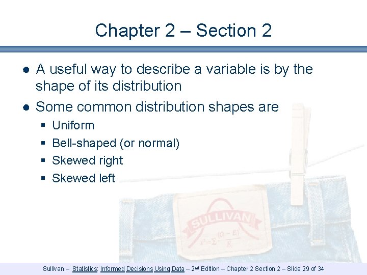
Chapter 2 – Section 2 ● A useful way to describe a variable is by the shape of its distribution ● Some common distribution shapes are § § Uniform Bell-shaped (or normal) Skewed right Skewed left Sullivan – Statistics: Informed Decisions Using Data – 2 nd Edition – Chapter 2 Section 2 – Slide 29 of 34

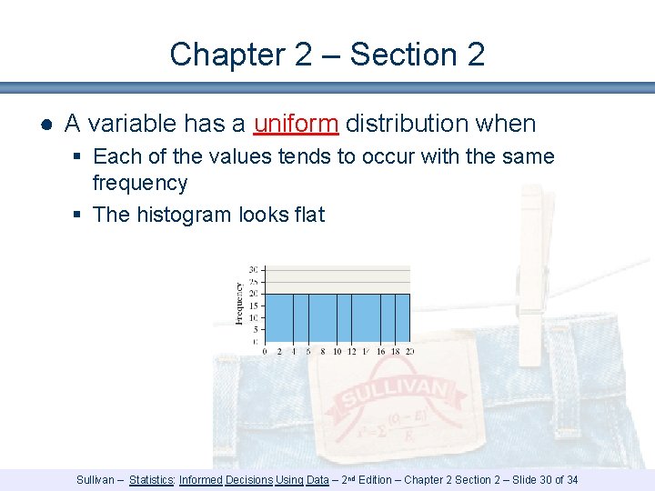
Chapter 2 – Section 2 ● A variable has a uniform distribution when § Each of the values tends to occur with the same frequency § The histogram looks flat Sullivan – Statistics: Informed Decisions Using Data – 2 nd Edition – Chapter 2 Section 2 – Slide 30 of 34

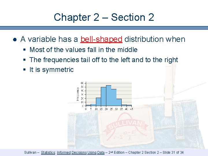
Chapter 2 – Section 2 ● A variable has a bell-shaped distribution when § Most of the values fall in the middle § The frequencies tail off to the left and to the right § It is symmetric Sullivan – Statistics: Informed Decisions Using Data – 2 nd Edition – Chapter 2 Section 2 – Slide 31 of 34

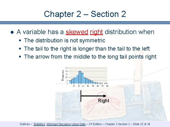
Chapter 2 – Section 2 ● A variable has a skewed right distribution when § The distribution is not symmetric § The tail to the right is longer than the tail to the left § The arrow from the middle to the long tail points right Right Sullivan – Statistics: Informed Decisions Using Data – 2 nd Edition – Chapter 2 Section 2 – Slide 32 of 34

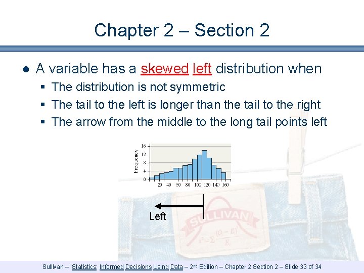
Chapter 2 – Section 2 ● A variable has a skewed left distribution when § The distribution is not symmetric § The tail to the left is longer than the tail to the right § The arrow from the middle to the long tail points left Left Sullivan – Statistics: Informed Decisions Using Data – 2 nd Edition – Chapter 2 Section 2 – Slide 33 of 34

Summary: Chapter 2 – Section 2 ● Quantitative data can be organized in several ways § Histograms based on data values are good for discrete data § Histograms based on classes (intervals) are good for continuous data § The shape of a distribution describes a variable … histograms are useful for identifying the shapes Sullivan – Statistics: Informed Decisions Using Data – 2 nd Edition – Chapter 2 Section 2 – Slide 34 of 34