Chapter 2 Probability and Risk What Is Risk

Chapter 2 Probability and Risk

What Is Risk In Finance? Risk can refer to 1. Uncertainty, 2. Volatility, 3. Bad outcomes (e. g. , bankruptcy), 4. Probability of bad outcomes, 5. Extent of bad outcomes, 6. Certainty of bad outcomes, etc.
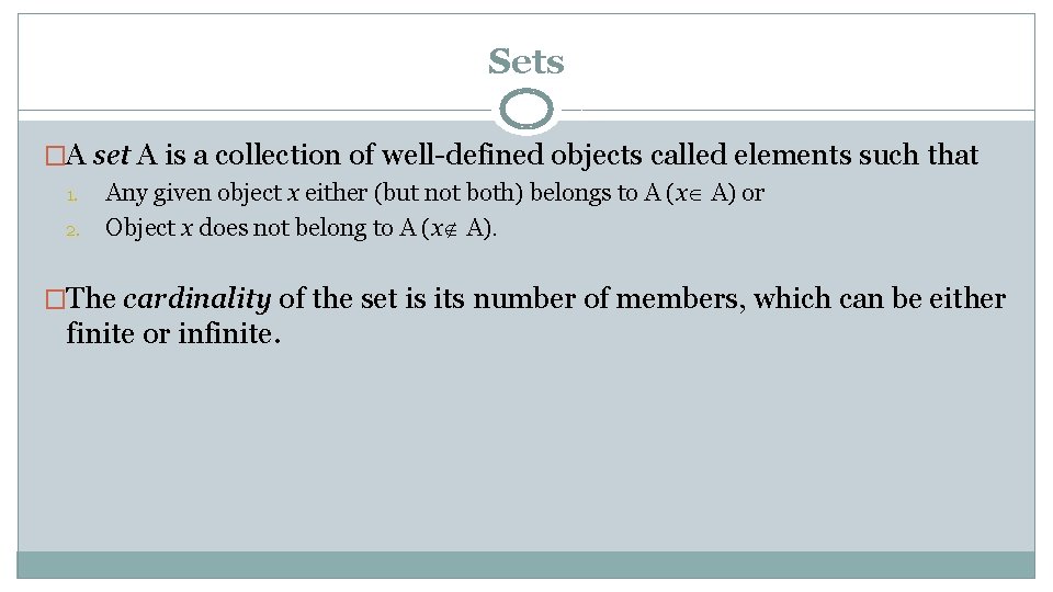
Sets �A set A is a collection of well-defined objects called elements such that 1. 2. Any given object x either (but not both) belongs to A (x A) or Object x does not belong to A (x A). �The cardinality of the set is its number of members, which can be either finite or infinite.
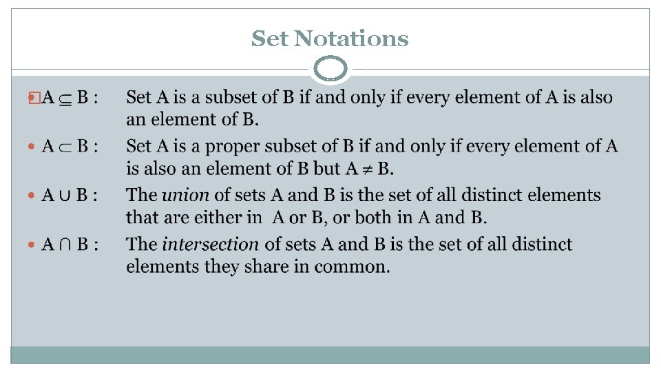
Set Notations �
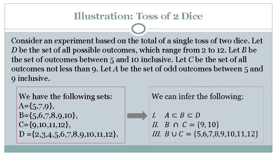
Illustration: Toss of 2 Dice Consider an experiment based on the total of a single toss of two dice. Let D be the set of all possible outcomes, which range from 2 to 12. Let B be the set of outcomes between 5 and 10 inclusive. Let C be the set of all outcomes not less than 9. Let A be the set of odd outcomes between 5 and 9 inclusive. We have the following sets: A={5, 7, 9}, B={5, 6, 7, 8, 9, 10}, C={9, 10, 11, 12}, D ={2, 3, 4, 5, 6, 7, 8, 9, 10, 11, 12}.
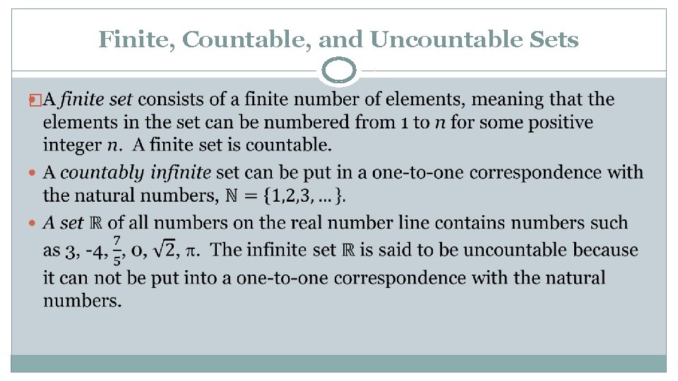
Finite, Countable, and Uncountable Sets �
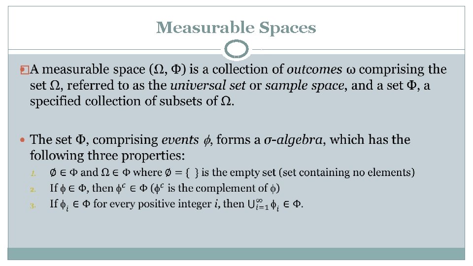
Measurable Spaces �
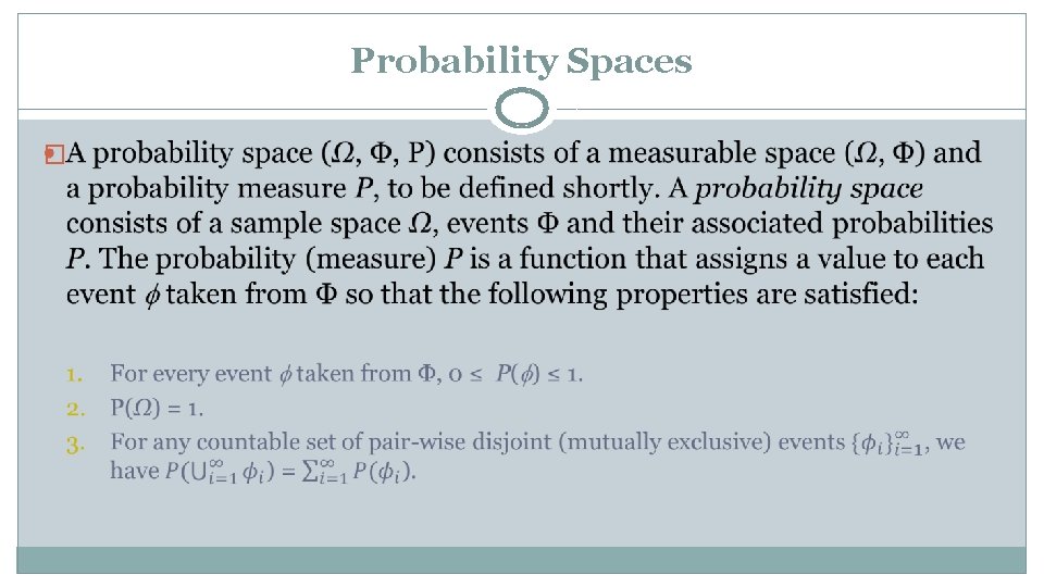
Probability Spaces �
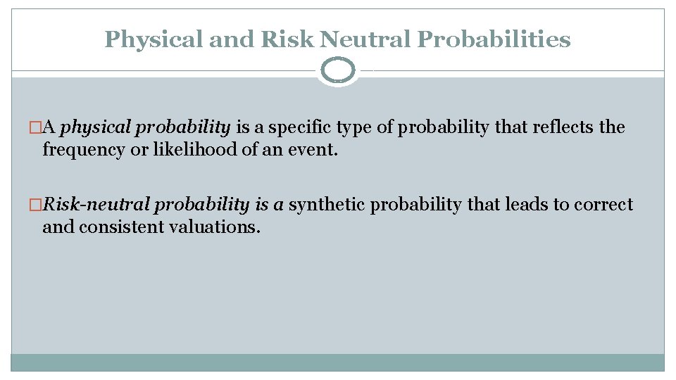
Physical and Risk Neutral Probabilities �A physical probability is a specific type of probability that reflects the frequency or likelihood of an event. �Risk-neutral probability is a synthetic probability that leads to correct and consistent valuations.
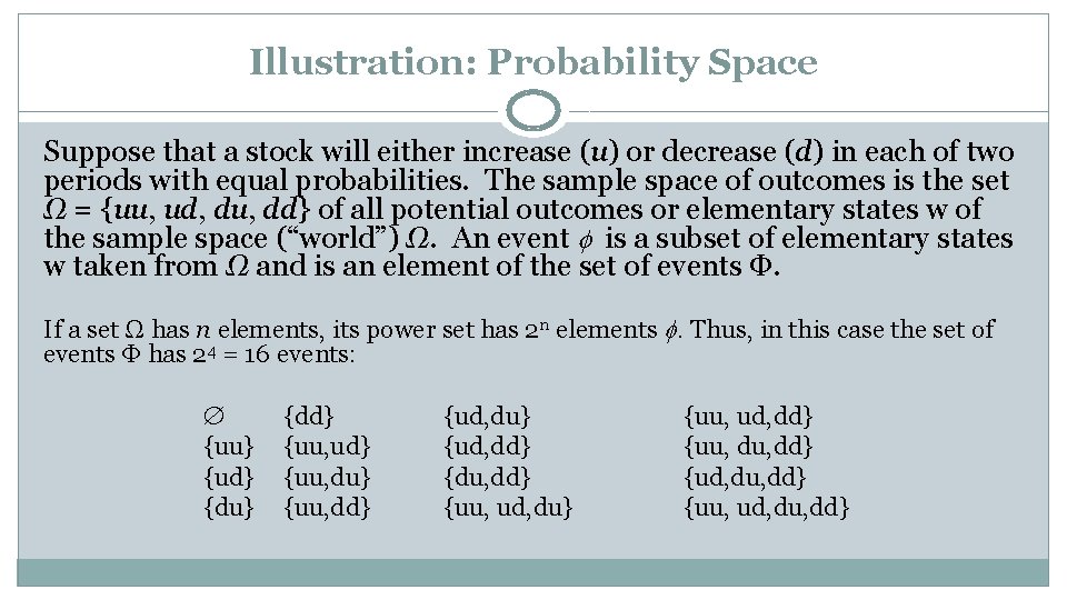
Illustration: Probability Space Suppose that a stock will either increase (u) or decrease (d) in each of two periods with equal probabilities. The sample space of outcomes is the set Ω = {uu, ud, du, dd} of all potential outcomes or elementary states w of the sample space (“world”) Ω. An event is a subset of elementary states w taken from Ω and is an element of the set of events Φ. If a set Ω has n elements, its power set has 2 n elements . Thus, in this case the set of events Ф has 24 = 16 events: {dd} {ud, du} {uu, ud, dd} {uu, ud} {ud, dd} {uu, du} {du, dd} {ud, du, dd} {du} {uu, dd} {uu, ud, du, dd}
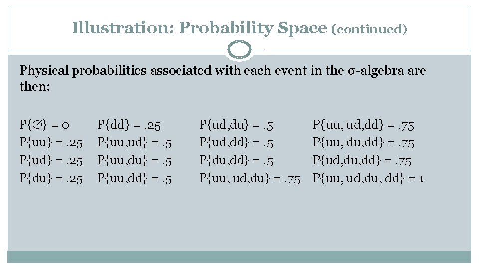
Illustration: Probability Space (continued) Physical probabilities associated with each event in the σ-algebra are then: P{ } = 0 P{uu} =. 25 P{ud} =. 25 P{du} =. 25 P{dd} =. 25 P{uu, ud} =. 5 P{uu, du} =. 5 P{uu, dd} =. 5 P{ud, du} =. 5 P{ud, dd} =. 5 P{du, dd} =. 5 P{uu, ud, du} =. 75 P{uu, ud, dd} =. 75 P{uu, dd} =. 75 P{ud, du, dd} =. 75 P{uu, ud, du, dd} = 1
Random Variables �A random variable X defined on a probability space (Ω, Φ, P) is a function from the set Ω of outcomes to ℝ (the set of real numbers) or a subset of the real numbers. �A random variable X is said to be discrete if it can assume at most a countable number of possible values: x 1, x 2, x 3, …. �A random variable X is said to be continuous if it can assume any value on a continuous range on the real number line.
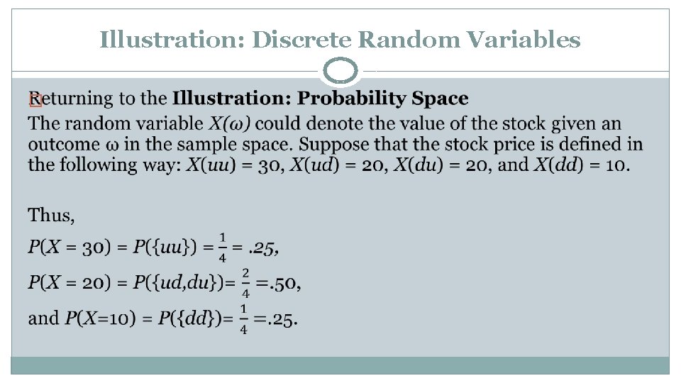
Illustration: Discrete Random Variables �
Metrics in Discrete Spaces �Expected Value �Variance and Standard Deviation �Co-movement Statistics: 1. Covariance 2. Coefficient of Correlation
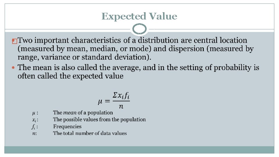
Expected Value �
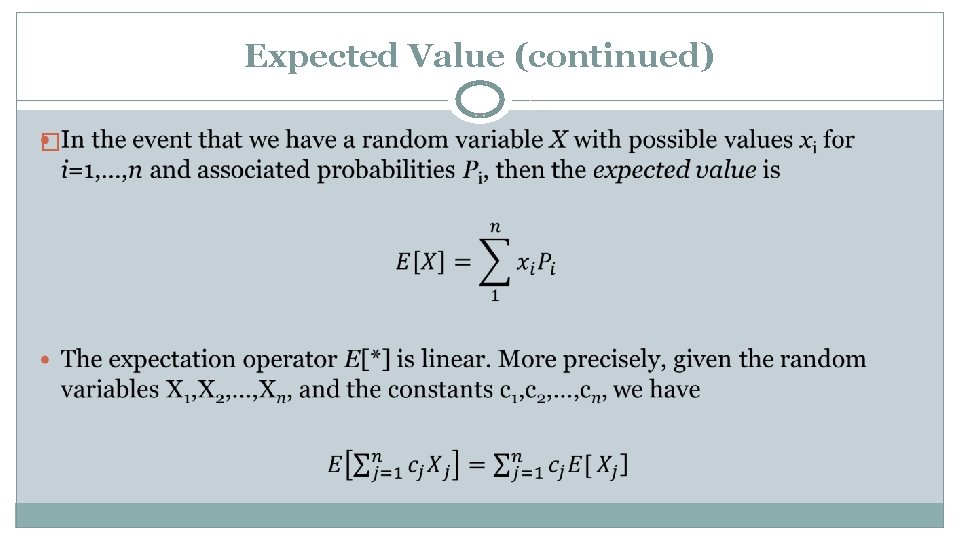
Expected Value (continued) �
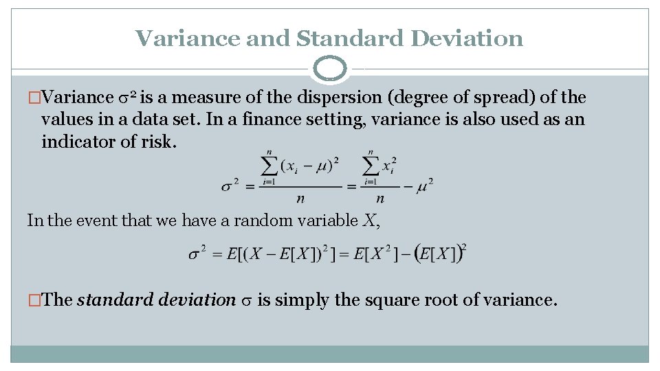
Variance and Standard Deviation �Variance 2 is a measure of the dispersion (degree of spread) of the values in a data set. In a finance setting, variance is also used as an indicator of risk. In the event that we have a random variable X, �The standard deviation is simply the square root of variance.
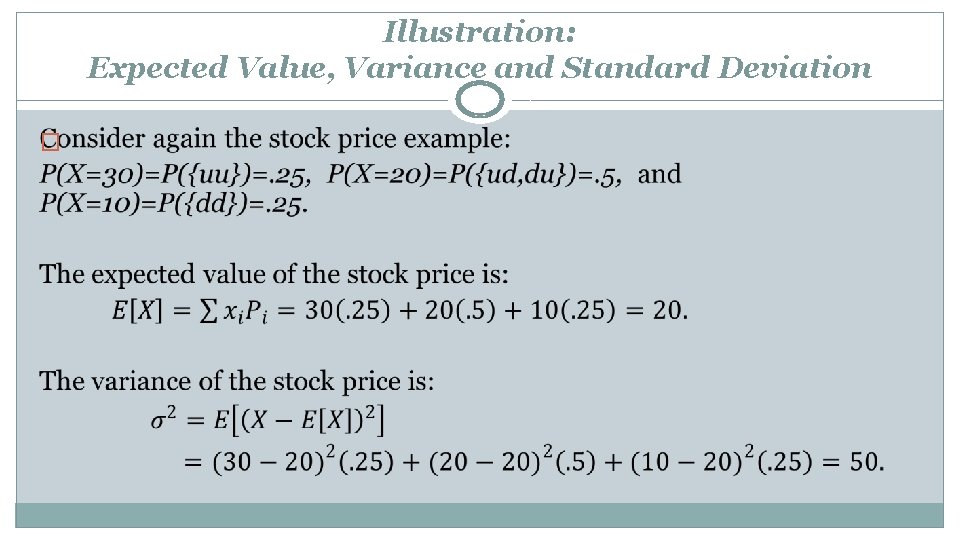
Illustration: Expected Value, Variance and Standard Deviation �
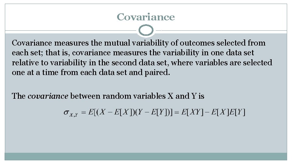
Covariance measures the mutual variability of outcomes selected from each set; that is, covariance measures the variability in one data set relative to variability in the second data set, where variables are selected one at a time from each data set and paired. The covariance between random variables X and Y is
Covariance (continued) Interpretations of Covariance: 1. The sign associated with the covariance indicates whether the relationship associated with the random variables are direct (positive sign) or inverse (negative sign). 2. If data sets are unrelated, the covariance is zero
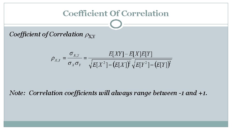
Coefficient Of Correlation Coefficient of Correlation X, Y Note: Correlation coefficients will always range between -1 and +1.
Coefficient of Correlation (continued) Interpretations of Coefficient of Correlation: �A correlation coefficient indicates the degree of the linear relationship between the variables X and Y. �A correlation coefficient of -1 means that there is a perfect linear relationship and that as the X values increase the Y values decrease on the line (negative slope). �A correlation coefficient of +1 means that there is a perfect linear relationship and that as the X values increase the Y values also increase on the line (positive slope). �A correlation coefficient equal to zero implies no linear relationship between the two random variables.

Metrics in Continuous Spaces �Probability Density Function �Cumulative Density Function �The Mean And Variance
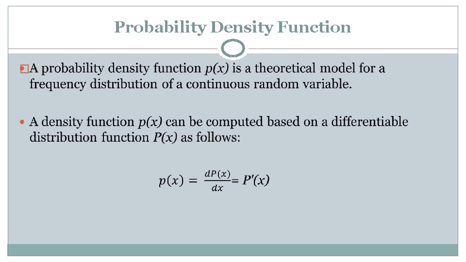
Probability Density Function �
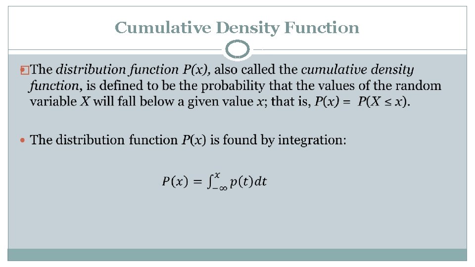
Cumulative Density Function �
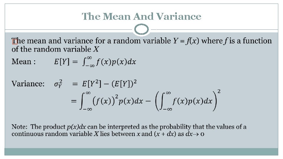
The Mean And Variance �
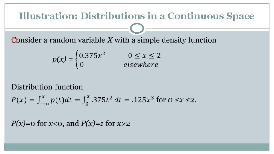
Illustration: Distributions in a Continuous Space �
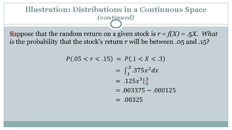
Illustration: Distributions in a Continuous Space (continued) �
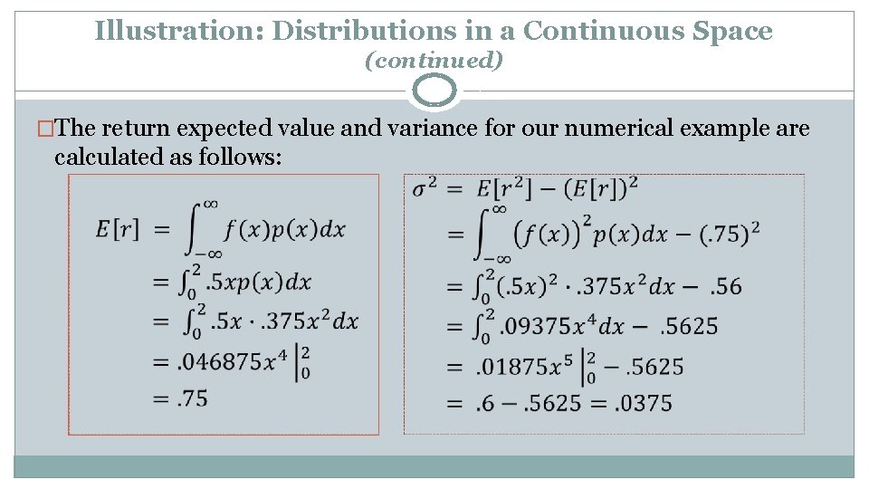
Illustration: Distributions in a Continuous Space (continued) �The return expected value and variance for our numerical example are calculated as follows:
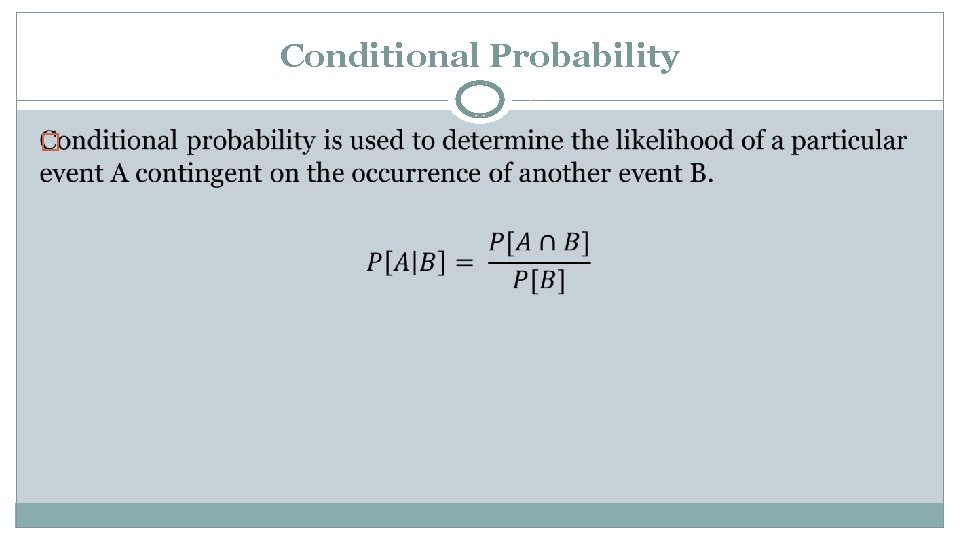
Conditional Probability �
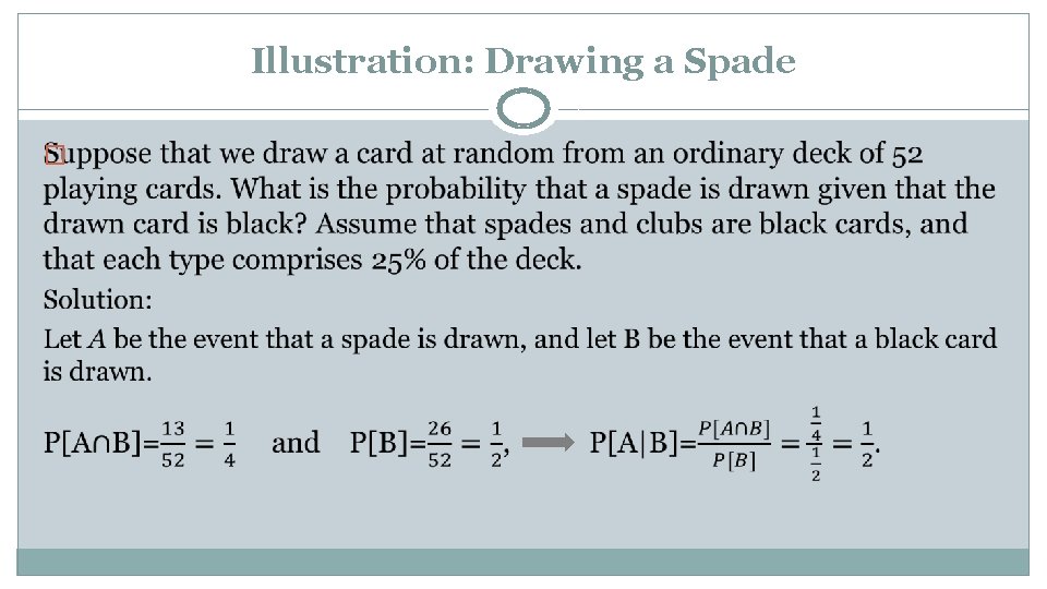
Illustration: Drawing a Spade �
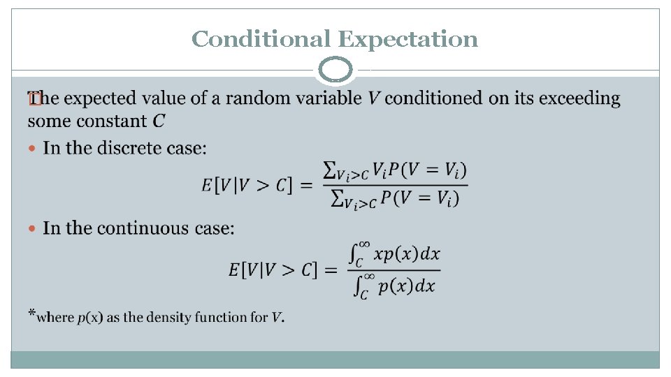
Conditional Expectation �
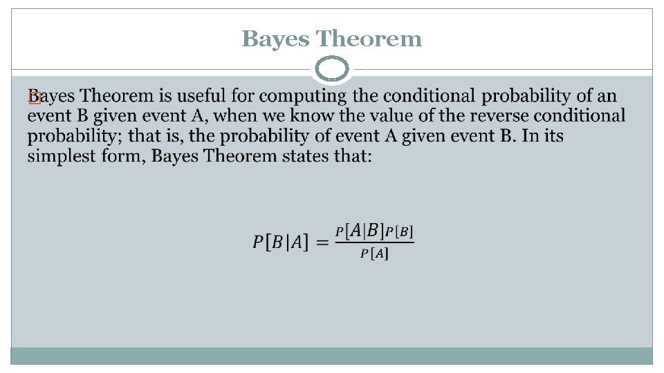
Bayes Theorem �
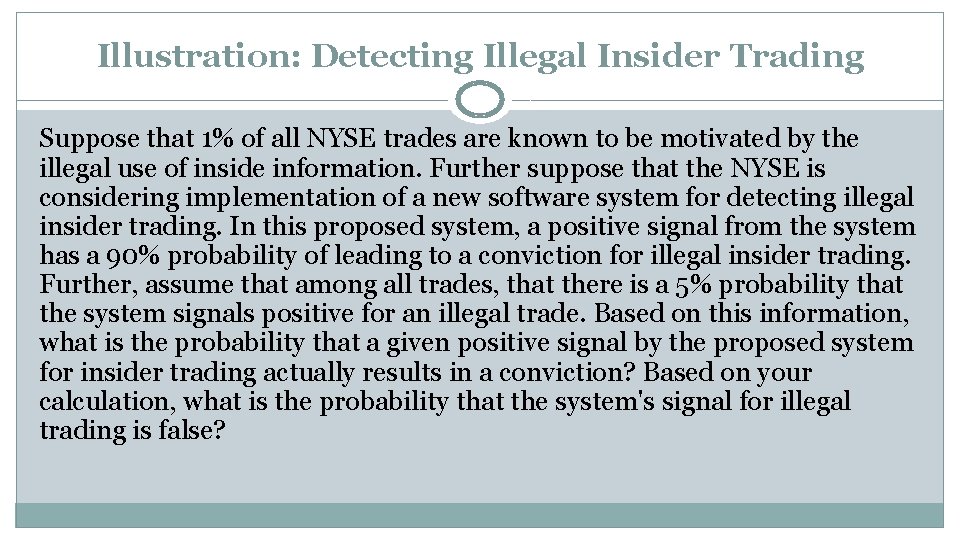
Illustration: Detecting Illegal Insider Trading Suppose that 1% of all NYSE trades are known to be motivated by the illegal use of inside information. Further suppose that the NYSE is considering implementation of a new software system for detecting illegal insider trading. In this proposed system, a positive signal from the system has a 90% probability of leading to a conviction for illegal insider trading. Further, assume that among all trades, that there is a 5% probability that the system signals positive for an illegal trade. Based on this information, what is the probability that a given positive signal by the proposed system for insider trading actually results in a conviction? Based on your calculation, what is the probability that the system's signal for illegal trading is false?
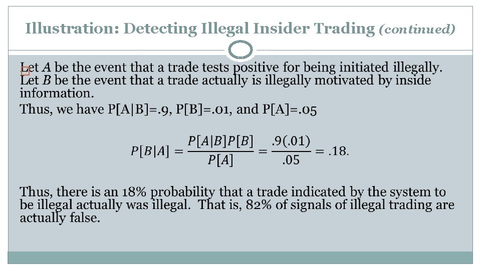
Illustration: Detecting Illegal Insider Trading (continued) �
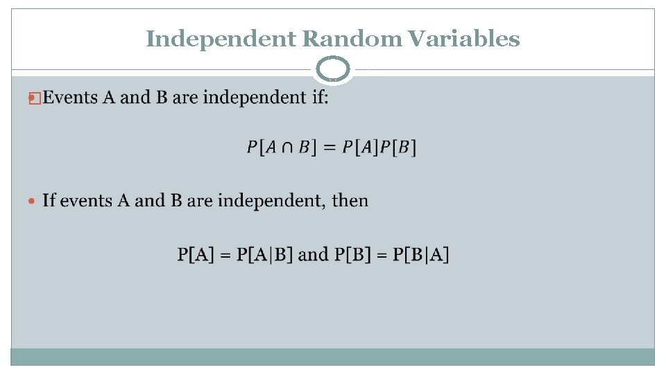
Independent Random Variables �
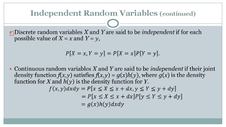
Independent Random Variables (continued) �
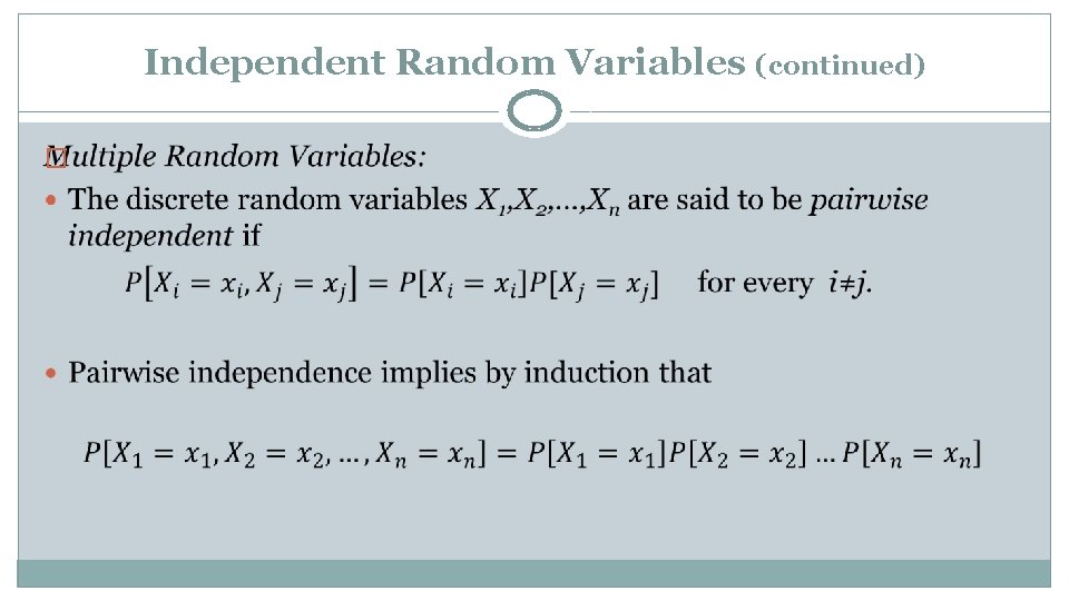
Independent Random Variables (continued) �
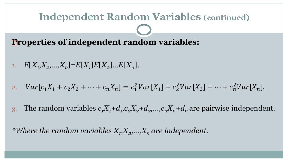
Independent Random Variables (continued) �
Distributions and Probability Density Functions �A probability distribution is a function that assigns a probability to each possible outcome in an experiment involving chance producing a discrete random variable. In the case of a continuous random variable, a probability density function is used to obtain probabilities of events.
Bernoulli Trial �Suppose that a random trial (or experiment) with two possible outcomes, one of which is called a “success” and the other a “failure, ” is performed. We define variable X=1 when the outcome is a success and define X=0 when the outcome is a failure. Suppose that the probability of success is p, with 0 ≤p≤ 1, such that P[X = 1]=p and P[X = 0]=1 -p. This random variable X is called a Bernoulli trial or process.
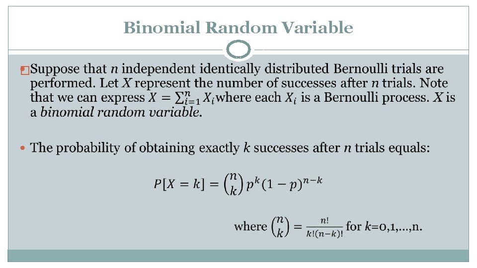
Binomial Random Variable �
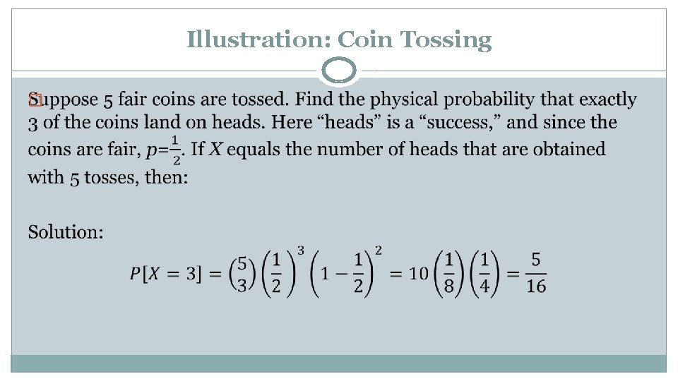
Illustration: Coin Tossing �
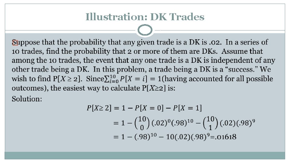
Illustration: DK Trades �
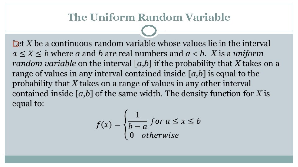
The Uniform Random Variable �
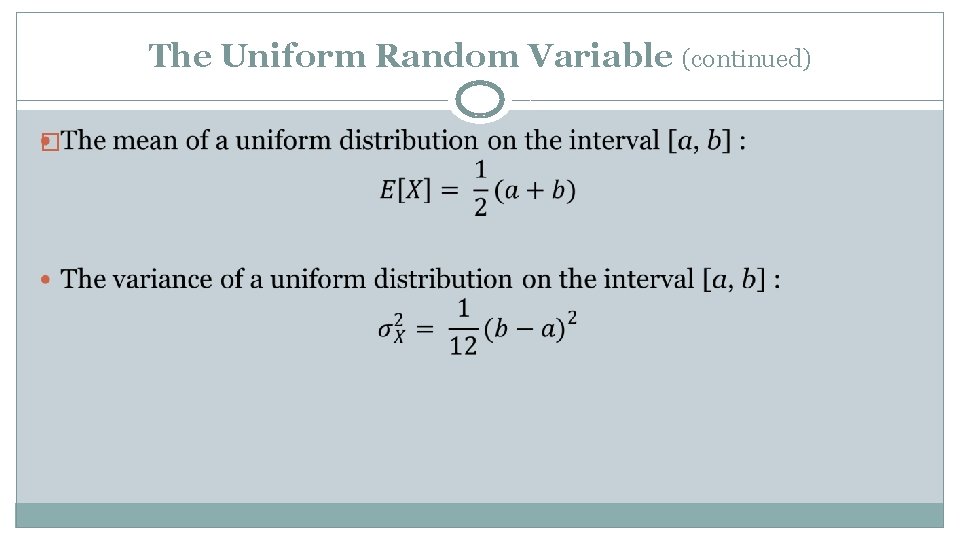
The Uniform Random Variable (continued) �
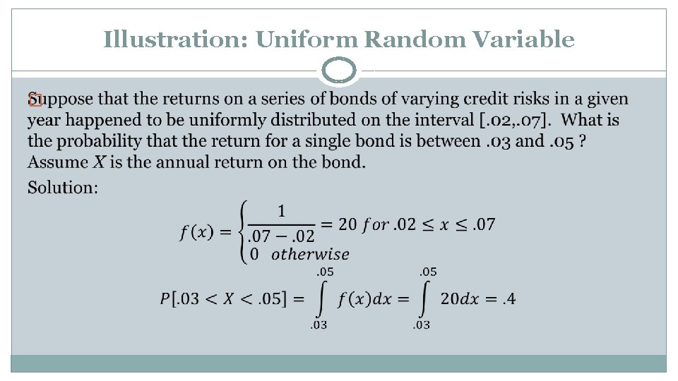
Illustration: Uniform Random Variable �
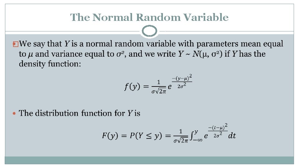
The Normal Random Variable �
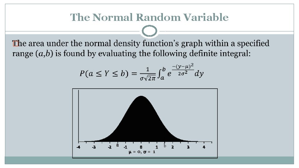
The Normal Random Variable � a b = 0, = 1
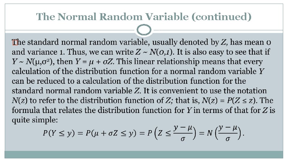
The Normal Random Variable (continued) �
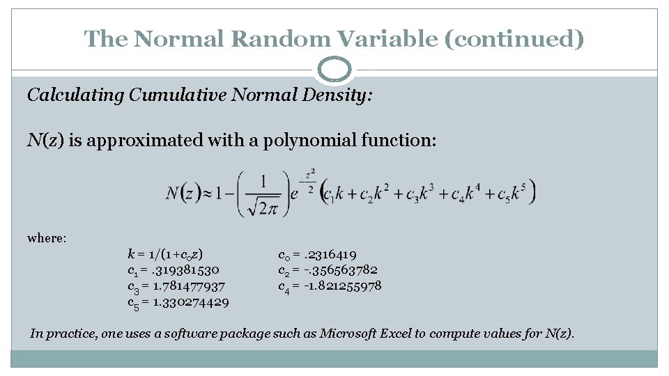
The Normal Random Variable (continued) Calculating Cumulative Normal Density: N(z) is approximated with a polynomial function: where: k = 1/(1+c 0 z) c 1 =. 319381530 c 3 = 1. 781477937 c 5 = 1. 330274429 c 0 =. 2316419 c 2 = -. 356563782 c 4 = -1. 821255978 In practice, one uses a software package such as Microsoft Excel to compute values for N(z).
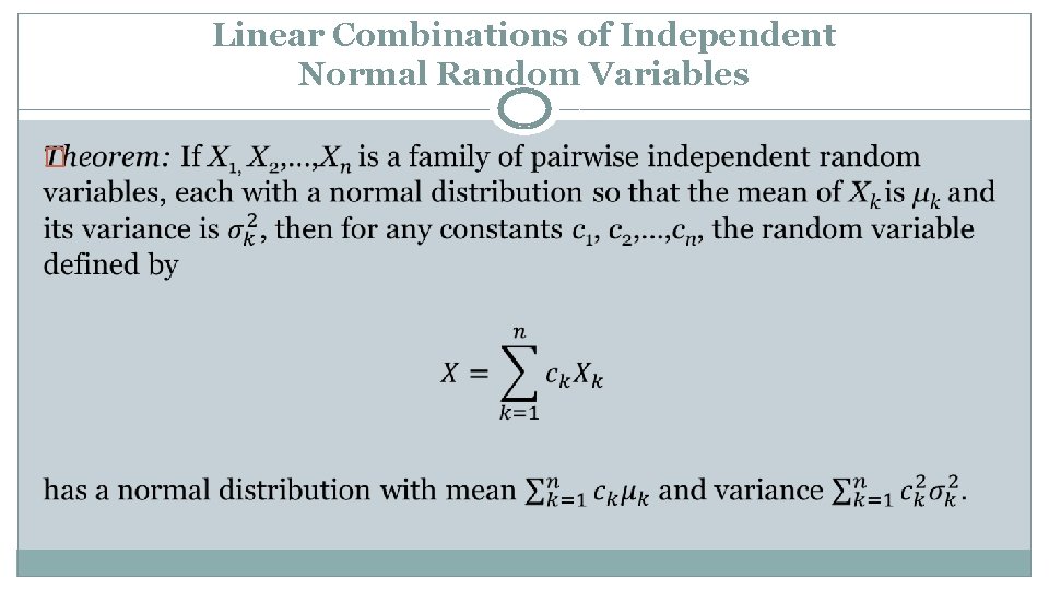
Linear Combinations of Independent Normal Random Variables �
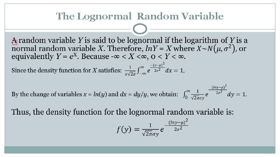
The Lognormal Random Variable �
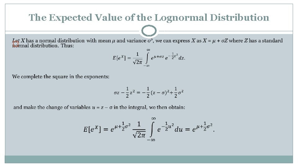
The Expected Value of the Lognormal Distribution �
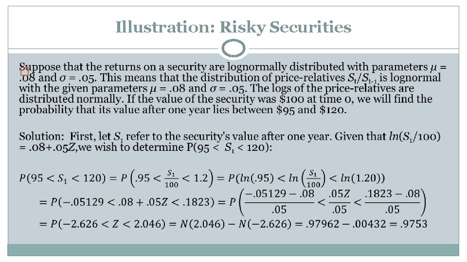
Illustration: Risky Securities �
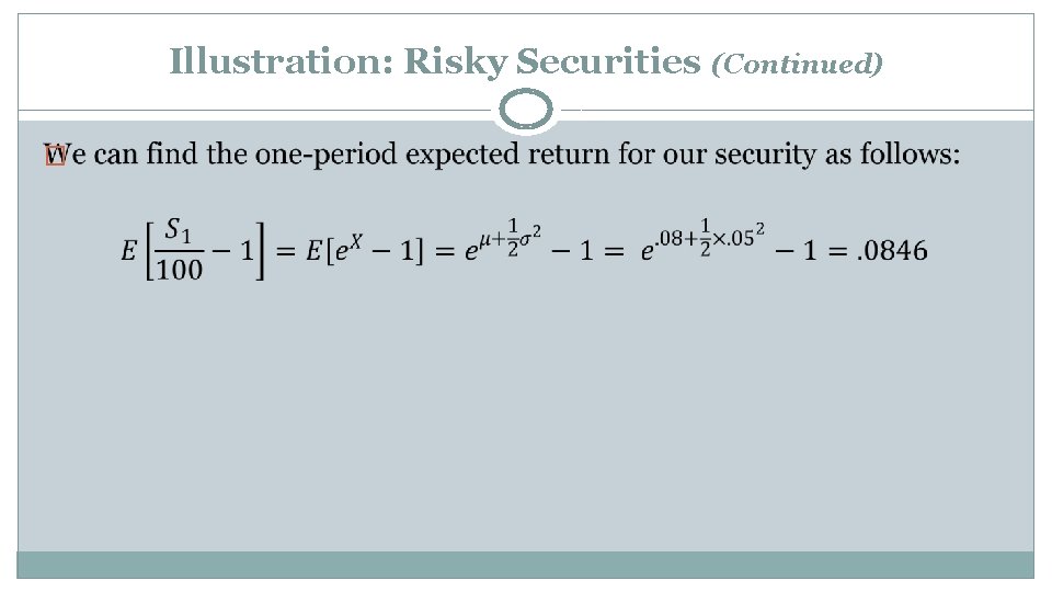
Illustration: Risky Securities (Continued) �
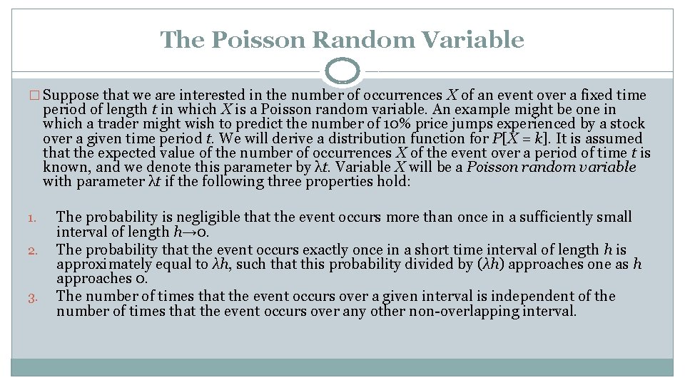
The Poisson Random Variable � Suppose that we are interested in the number of occurrences X of an event over a fixed time period of length t in which X is a Poisson random variable. An example might be one in which a trader might wish to predict the number of 10% price jumps experienced by a stock over a given time period t. We will derive a distribution function for P[X = k]. It is assumed that the expected value of the number of occurrences X of the event over a period of time t is known, and we denote this parameter by λt. Variable X will be a Poisson random variable with parameter λt if the following three properties hold: 1. 2. 3. The probability is negligible that the event occurs more than once in a sufficiently small interval of length h→ 0. The probability that the event occurs exactly once in a short time interval of length h is approximately equal to λh, such that this probability divided by (λh) approaches one as h approaches 0. The number of times that the event occurs over a given interval is independent of the number of times that the event occurs over any other non-overlapping interval.
![Deriving the Poisson Distribution Suppose that we divide the time interval [T, T+t] into Deriving the Poisson Distribution Suppose that we divide the time interval [T, T+t] into](http://slidetodoc.com/presentation_image_h/3334089bf3f758276a4ea1354afb5c59/image-58.jpg)
Deriving the Poisson Distribution Suppose that we divide the time interval [T, T+t] into n subintervals of equal length so that the ith interval takes the form [T+t(i-1)/n, T+ti/n] for i=1, …, n. By property 1 , the probability that the event occurs more than once in the ith time interval is negligible if n is large. By property 2, the probability that the event occurs in the ith time interval is approximately p=λt/n for i =1, …, n. Thus, the Poisson process follows a Bernoulli process within each of the n time intervals, with probability p=λt/n of success and probability 1 -p=1 -λt/n of failure. Furthermore, by property 3, we can regard the Poisson process as approximating n independent identically distributed Bernoulli processes. Thus, the process follows a binomial distribution with n trials and p=λt/n.
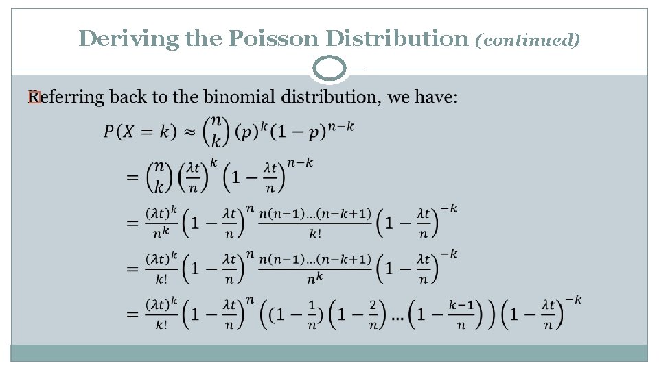
Deriving the Poisson Distribution (continued) �
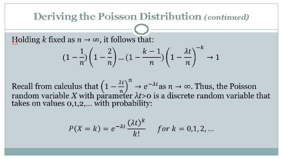
Deriving the Poisson Distribution (continued) �
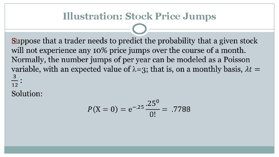
Illustration: Stock Price Jumps �
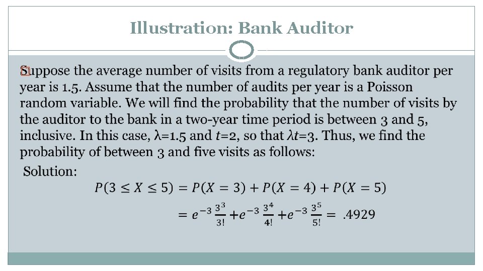
Illustration: Bank Auditor �
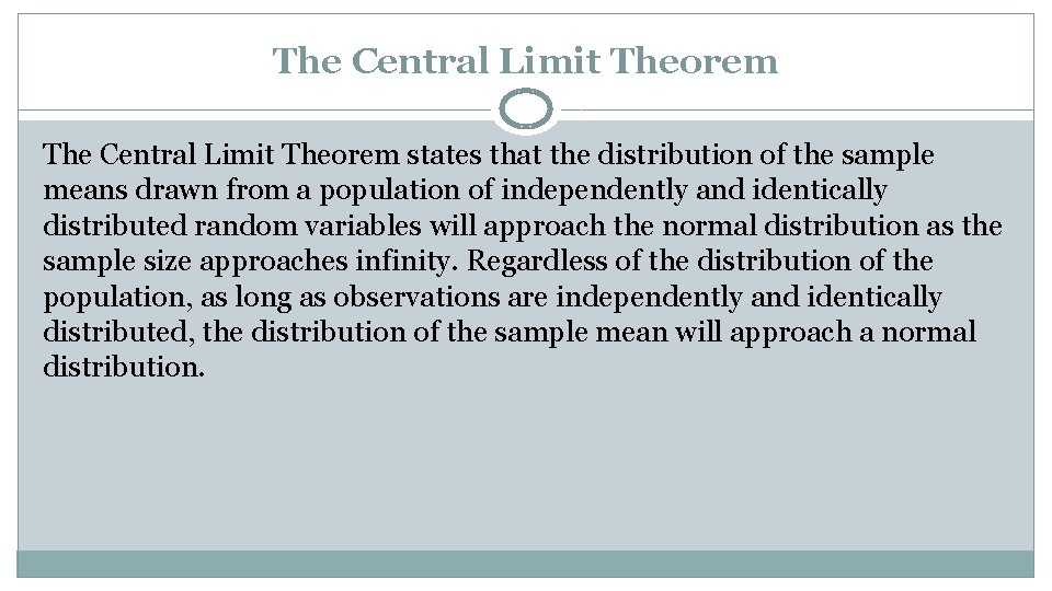
The Central Limit Theorem states that the distribution of the sample means drawn from a population of independently and identically distributed random variables will approach the normal distribution as the sample size approaches infinity. Regardless of the distribution of the population, as long as observations are independently and identically distributed, the distribution of the sample mean will approach a normal distribution.
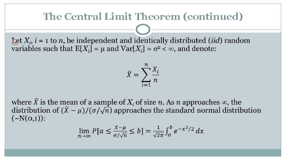
The Central Limit Theorem (continued) �
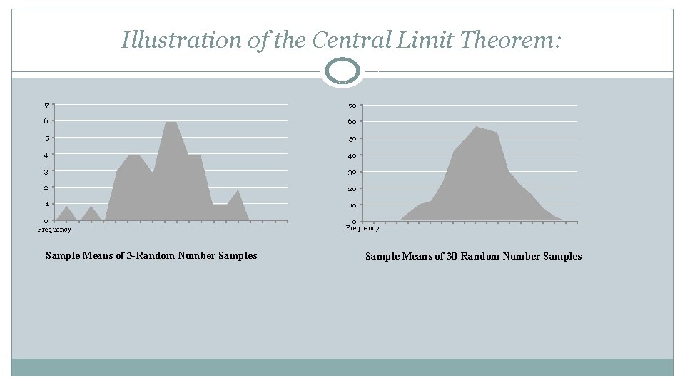
Illustration of the Central Limit Theorem: 7 70 6 60 5 50 4 40 3 30 2 20 1 10 0 Frequency Sample Means of 3 -Random Number Samples 0 Frequency Sample Means of 30 -Random Number Samples
Joint Probability Distributions �We have been studying probability from the perspective of a single random variable. Often, one is interested in the probabilistic behavior of two (or more) random variables studied jointly.
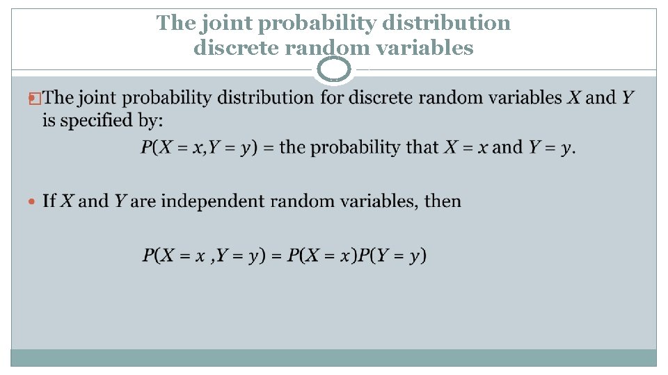
The joint probability distribution discrete random variables �
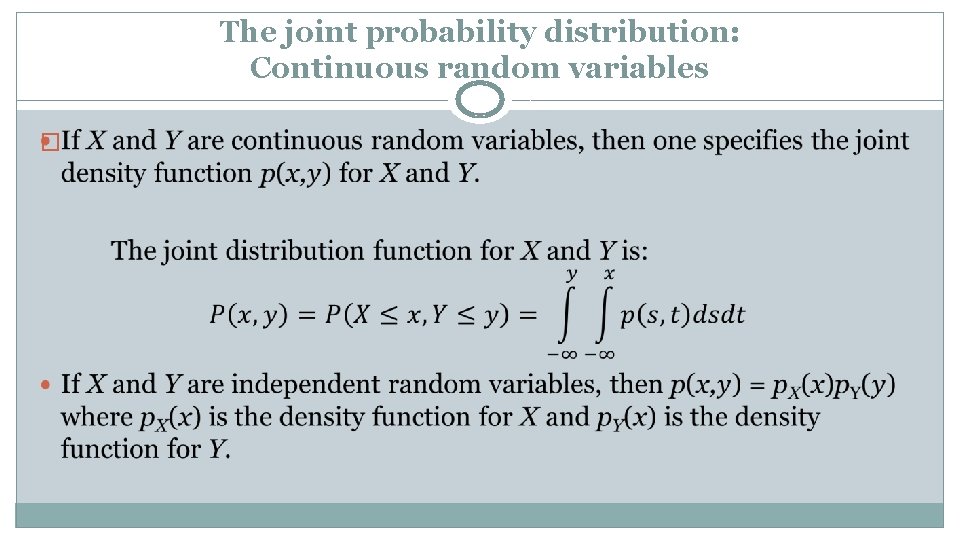
The joint probability distribution: Continuous random variables �
Illustration: Transaction Execution Delay Suppose that X is the amount of time that it takes for a security’s transaction to transmit from a hedge fund to a stock exchange. Assume that this time delay has a uniform distribution from 0 to 20 milliseconds. Let Y be the amount of time required for the stock exchange to actually execute the transaction once received. Assume this time has a uniform distribution from 0 to 10 milliseconds. Also assume that the random variables X and Y are independent. Determine the probability that the total transaction completion time (transmission and execution) is less than 10 milliseconds.
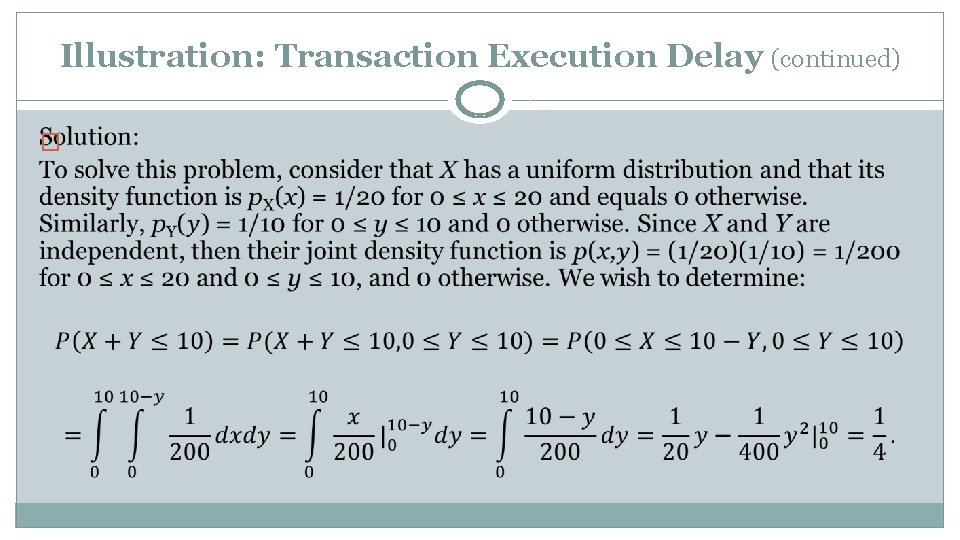
Illustration: Transaction Execution Delay (continued) �
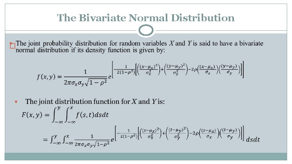
The Bivariate Normal Distribution �
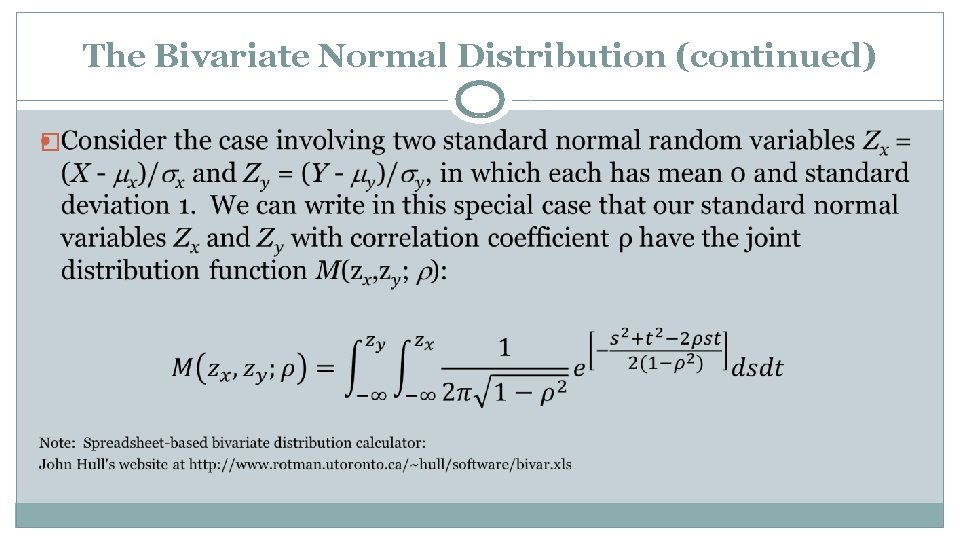
The Bivariate Normal Distribution (continued) �
Illustration: Calculating Bivariate Normal Densities �Suppose that the log of one stock’s price relative Xt =ln(St /St-1) is distributed normally with mean 5% and standard deviation 1%. The log of another stock’s price relative Yt =ln(St /St-1) is distributed normally with mean 6% and standard deviation 2%. Assume that Xt and Yt have a bivariate normal distribution and that their correlation coefficient is ρ = . 5. Find the probability of the event that the first stock’s return is less than 6. 5% and the second stock’s return is less than 6. 6%.
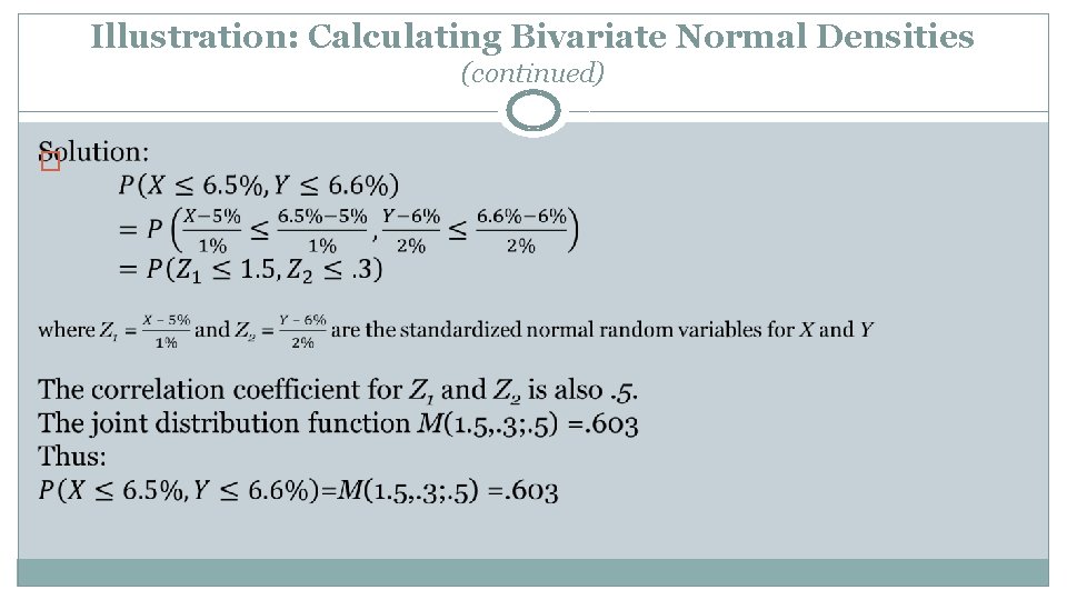
Illustration: Calculating Bivariate Normal Densities (continued) �
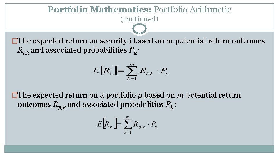
Portfolio Mathematics: Portfolio Arithmetic (continued) �The expected return on security i based on m potential return outcomes Ri, k and associated probabilities Pk : �The expected return on a portfolio p based on m potential return outcomes Rp, k and associated probabilities Pk :
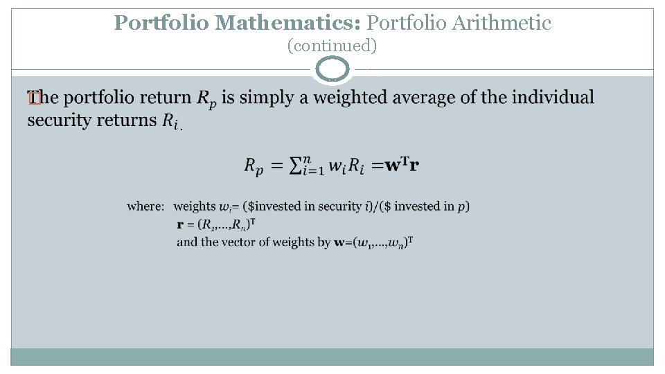
Portfolio Mathematics: Portfolio Arithmetic (continued) �
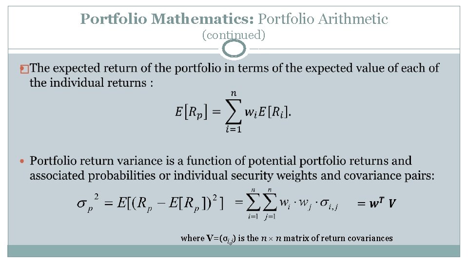
Portfolio Mathematics: Portfolio Arithmetic (continued) � where V=(σi, j) is the n × n matrix of return covariances
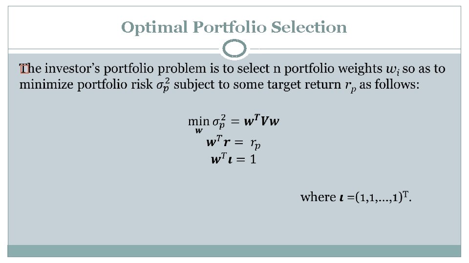
Optimal Portfolio Selection �
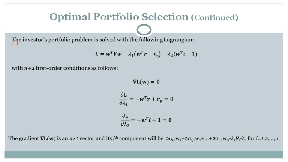
Optimal Portfolio Selection (Continued) �
Portfolio Selection Illustration Suppose that an investor wishes to comprise the lowest risk portfolio of three assets. The expected returns of the three assets A, B and C are. 1, . 2 and. 3, respectively. Their standard deviations are. 2, . 3 and. 4. The returns covariance between assets A and B is. 03, the returns covariance between assets A and C is. 04 and the returns covariance between assets B and C is. 06. What should be the weights of this optimal or lowest risk portfolio if he seeks an expected portfolio return of 15%?
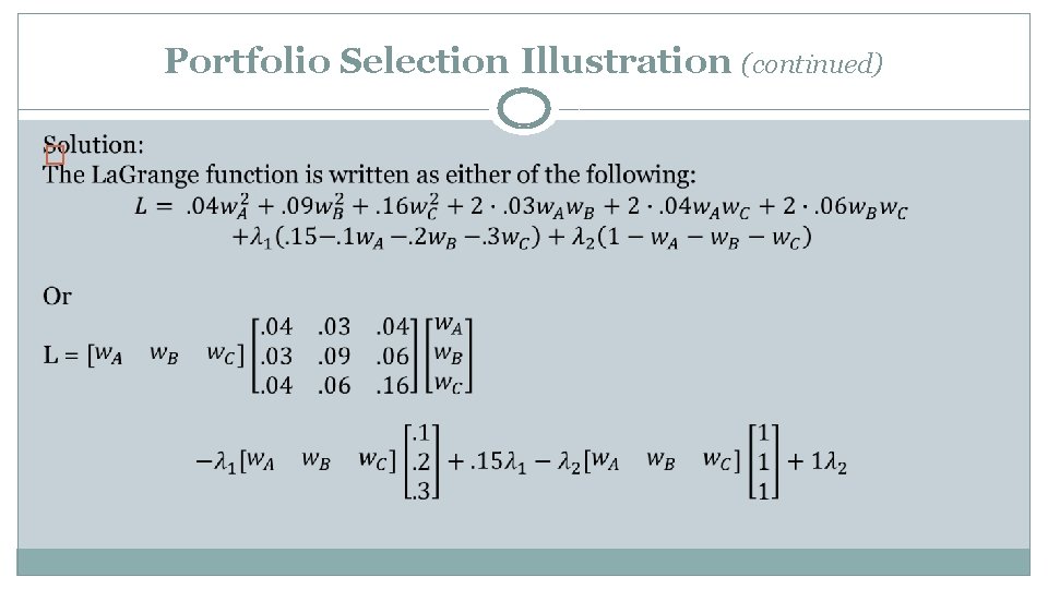
Portfolio Selection Illustration (continued) �
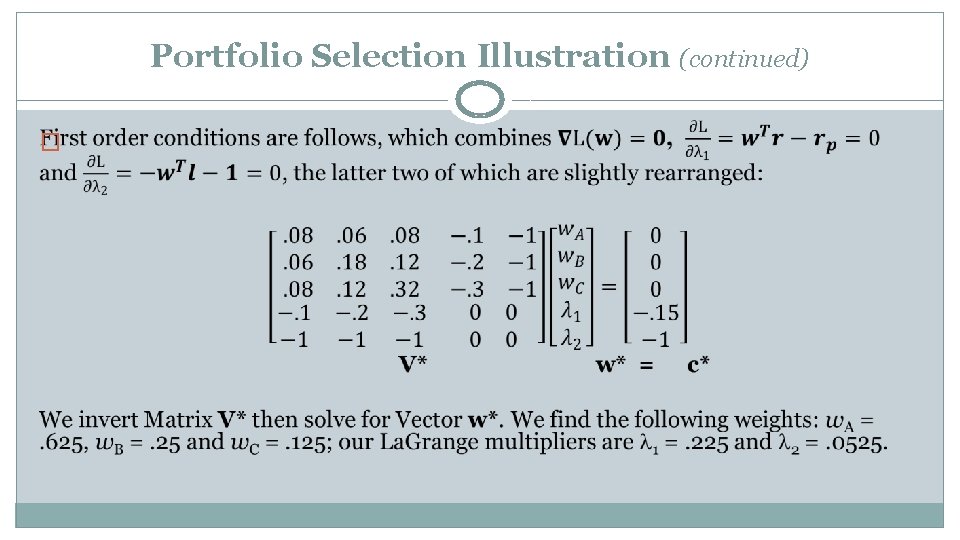
Portfolio Selection Illustration (continued) �
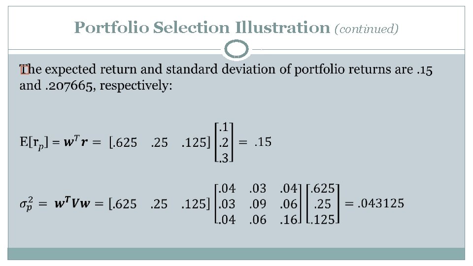
Portfolio Selection Illustration (continued) �
- Slides: 83